Normal Approximation in R-code
| ✅ Paper Type: Free Essay | ✅ Subject: Statistics |
| ✅ Wordcount: 1233 words | ✅ Published: 04 Oct 2017 |
Normal approximation using R-code
Abstract
The purpose of this research is to determine when it is more desirable to approximate a discrete distribution with a normal distribution. Particularly, it is more convenient to replace the binomial distribution with the normal when certain conditions are met. Remember, though, that the binomial distribution is discrete, while the normal distribution is continuous. The aim of this study is also to have an overview on how normal distribution can also be concerned and applicable in the approximation of Poisson distribution. The common reason for these phenomenon depends on the notion of a sampling distribution. I also provide an overview on how Binomial probabilities can be easily calculated by using a very straightforward formula to find the binomial coefficient. Unfortunately, due to the factorials in the formula, it can easily lead into computational difficulties with the binomial formula. The solution is that normal approximation allows us to bypass any of these problems.
Introduction
The shape of the binomial distribution changes considerably according to its parameters, n and p. If the parameter p, the probability of “success” (or a defective item or a failure) in a single experimental, is sufficiently small (or if q = 1 – p is adequately small), the distribution is usually asymmetrical. Alternatively, if p is sufficiently close enough to 0.5 and n is sufficiently large, the binomial distribution can be approximated using the normal distribution. Under these conditions the binomial distribution is approximately symmetrical and inclines toward a bell shape. A binomial distribution with very small p (or p very close to 1) can be approximated by a normal distribution if n is very large. If n is large enough, sometimes both the normal approximation and the Poisson approximation are applicable. In that case, use of the normal approximation is generally preferable since it allows easy calculation of cumulative probabilities using tables or other technology. When dealing with extremely large samples, it becomes very tedious to calculate certain probabilities. In such circumstances, using the normal distribution to approximate the exact probabilities of success is more applicable or otherwise it would have been achieved through laborious computations. For n sufficiently large (say n > 20) and p not too close to zero or 1 (say 0.05 < p < 0.95) the distribution approximately follows the Normal distribution.
To find the binomial probabilities, this can be used as follows:
If X ~ binomial (n,p) where n > 20 and 0.05 < p < 0.95 then approximately X has the Normal distribution with mean E(X) = np
 So
So  is approximately N(0,1).
R programming will be used for calculating probabilities associated with the binomial, Poisson, and normal distributions. Using R code, it will enable me to test the input and model the output in terms of graph. The system requirement for R is to be provided an operating system platform to be able to perform any calculation.

- Firstly, we are going to proceed by considering the conditions under which the discrete distribution inclines towards a normal distribution.
- Generating a set of the discrete distribution so that it inclines towards a bell shape. Or simply using R by just specifying the size needed.
- And lastly compare the generated distribution with the target normal distribution
Normal approximation of binomial probabilities
Let X ~ BINOM(100, 0.4).
Using R to compute Q = P(35 < X ≤ 45) = P(35.5 < X ≤ 45.5):
> diff(pbinom(c(45,35), 100, .4))
[1] -0.6894402
Whether it is for theoretical or practical purposes, Using Central Limit Theorem is more convenient to approximate the binomial probabilities.
When n is large and (np/q, nq/p) > 3, where q = 1 – p
The CLT states that, for situations where n is large,
Y ~ BINOM(n, p) is approximately NORM(μ = np, σ = [np(1 – p)]1/2).
Hence, using the first expression Q = P(35 < X ≤ 45)
The approximation results as follows:
l Φ(1.0206) – Φ(–1.0206) = 0.6926
Correction for continuity adjustment will be used in order for a continuous distribution to approximate a discrete. Recall that a random variable can take all real values within a range or interval while a discrete random variable can take on only specified values. Thus, using the normal distribution to approximate the binomial, more precise approximations of the probabilities are obtained.
After applying the continuity correction to Q = P(35.5 < X ≤ 45.5), it results to:
Φ(1.1227) – Φ(–0.91856) = 0.6900
We can verify the calculation using R,
> pnorm(c(1.1227))-pnorm(c(-0.91856))
[1] 0.6900547
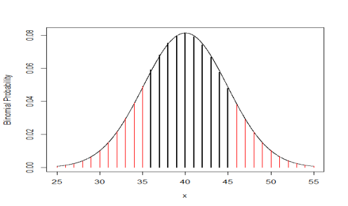
Below an alternate R code is used to plot and illustrate the normal approximation to binomial.
Let X ~ BINOM(100, l4) and P(35 < X  45)
45)
> pbinom(45, 100, .4) – pbinom(35, 100, .4)
[1] 0.6894402
# Normal approximation > pnorm(5/sqrt(24)) – pnorm(-5/sqrt(24))
[1] 0.6925658
# Applying Continuity Correction > pnorm(5.5/sqrt(24)) – pnorm(-4.5/sqrt(24))
[1] 0.6900506
x1=36:45
x2= c(25:35, 46:55)
x1x2= seq(25, 55, by=.01)
plot(x1x2, dnorm(x1x2, 40, sqrt(24)), type=”l”,
xlab=”x”, ylab=”Binomial Probability”)
lines(x2, dbinom(x2, 100, .4), type=”h”, col=2)
lines(x1, dbinom(x1, 100, .4), type=”h”, lwd=2)
Poisson approximation of binomial probabilities
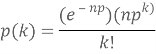
For situations in which p is very small with large n, the Poisson distribution can be used as an approximation to the binomial distribution. The larger the n and the smaller the p, the better is the approximation. The following formula for the Poisson model is used to approximate the binomial probabilities:
A Poisson approximation can be used when n is large (n>50) and p is small (p<0.1)
Then X~Po(np) approximately.
AN EXAMPLE
The probability of a person will develop an infection even after taking a vaccine that was supposed to prevent the infection is 0.03. In a simple random sample of 200 people in a community who get vaccinated, what is the probability that six or fewer person will be infected?
Solution:
Let X be the random variable of the number of people being infected. X follows a binomial probability distribution with n=200 and p= 0.03. The probability of having six or less people getting infected is
P (X ≤ 6 ) = 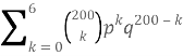
The probability is 0.6063. Calculation can be verified using R as
> sum(dbinom(0:6, 200, 0.03))
[1] 0.6063152
Or otherwise,
> pbinom(6, 200, .03)
[1] 0.6063152
In order to avoid such tedious calculation by hand, Poisson distribution or a normal distribution can be used to approximate the binomial probability.
Poisson approximation to the binomial distribution
To use Poisson distribution as an approximation to the binomial probabilities, we can consider that the random variable X follows a Poisson distribution with rate λ=np= (200) (0.03) = 6. Now, we can calculate the probability of having six or fewer infections as
P (X ≤ 6) = 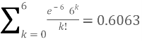
The results turns out to be similar as the one that has been obtained using the binomial distribution.
Calculation can be verified using R,
> ppois(6, lambda = 6)
[1] 0.6063028
It can be clearly seen that the Poisson approximation is very close to the exact probability.
The same probability can be calculated using the normal approximation. Since binomial distribution is for a discrete random variable and normal distribution for continuous, continuity correction is needed when using a normal distribution as an approximation to a discrete distribution.
For large n with np>5 and nq>5, a binomial random variable X with X∼Bin(n,p) can be approximated by a normal distribution with mean = np and variance = npq. i.e. X∼N(6,5.82).
The probability that there will be six or fewer cases of these incidences:
P (X≤6) = P (z ≤  )
)
As it was mentioned earlier, correction for continuity adjustment is needed. So, the above expression become
P (X≤6) = P (z ≤  )
)
= P (z ≤  )
)
= P (z ≤  )
)
Using R, the probability which is 0.5821 can be obtained:
> pnorm(0.2072)
[1] 0.5820732
It can be noted that the approximation used is close to the exact probability 0.6063. However, the Poisson distribution gives better approximation. But for larger sample sizes, where n is closer to 300, the normal approximation is as good as the Poisson approximation.
The normal approximation to the Poisson distribution
The normal distribution can also be used as an approximation to the Poisson distribution whenever the parameter λ is large
When λ is large (say λ>15), the normal distribution can be used as an approximation where
X~N(λ, λ)
Here also a continuity correction is needed, since a continuous distribution is used to approximate a discrete one.
Example
A radioactive disintegration gives counts that follow a Poisson distribution with a mean count of 25 per second. Find probability that in a one-second interval the count is between 23 and 27 inclusive.
Solution:
Let X be the radioactive count in one-second interval, X~Po(25)
Using normal approximation, X~N(25,25)
P(23≤x≤27) =P(22.5 =P ( =P (-0.5 < Z < 0.5) =0.383 (3 d.p) Using R: > pnorm(c(0.5))-pnorm(c(-0.5)) [1] 0.3829249 In this study it has been concluded that when using the normal distribution to approximate the binomial distribution, a more accurate approximations was obtained. Moreover, it turns out that as n gets larger, the Binomial distribution looks increasingly like the Normal distribution. The normal approximation to the binomial distribution is, in fact, a special case of a more general phenomenon. The importance of employing a correction for continuity adjustment has also been investigated. It has also been viewed that using R programming, more accurate outcome of the distribution are obtained. Furthermore a number of examples has also been analyzed in order to have a better perspective on the normal approximation. Using normal distribution as an approximation can be useful, however if these conditions are not met then the approximation may not be that good in estimating the probabilities. )
)
Cite This Work
To export a reference to this article please select a referencing stye below:
Related Services
View all


DMCA / Removal Request
If you are the original writer of this essay and no longer wish to have your work published on UKEssays.com then please click the following link to email our support team:
Request essay removal