Impact of Temperature on Viscosity of Liquid
| ✅ Paper Type: Free Essay | ✅ Subject: Physics |
| ✅ Wordcount: 2015 words | ✅ Published: 11 Sep 2017 |
INTRODUCTION
Hydrodynamics, as defined by the Merriam Webster Dictionary, is the ‘branch of physics that deals with the motion of fluids, and the forces acting on solid bodies immersed in fluids and in motion relative to them’ (2017). The study of fluids originated in Ancient Greece, was coupled with the works of Persian philosophers in Medieval times, and eventually, with many contributions made by scientists such as Archimedes, Leonardo Da Vinci and Isaac Newton, was developed into the branch of fluid dynamics that exists today (WiseGeek, 2017).
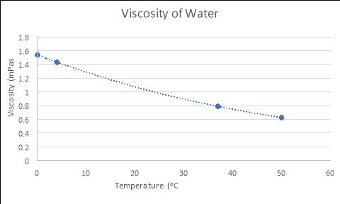
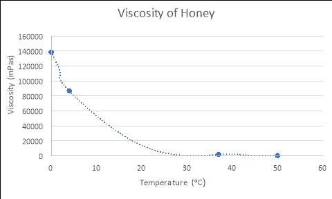
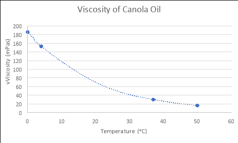
Any substance can be classed as a fluidif it ‘changes shape uniformly in response to external forces’. Many characteristics of such a substance include; pressure, temperature, mass, density and viscosity (Washington.edu, 2017). The term ‘viscosity’ is defined as ‘a fluid’s resistance to flow in relation to its inner molecular structure‘, and is largely affected by temperature (Viscopedia, 2017). As the temperature of a fluid increases, so does the thermal/kinetic energy of its liquid molecules, which results in increased amounts of movement as the particles begin to move faster. Due to this increased amount of movement, the attractive binding energy of the fluid is reduced, consequently decreasing the fluid’s resistance to flow (Azom, 2013). This principle is demonstrated in the following theoretical figures, which depict the relationship between the temperatures and viscosities of various fluids:
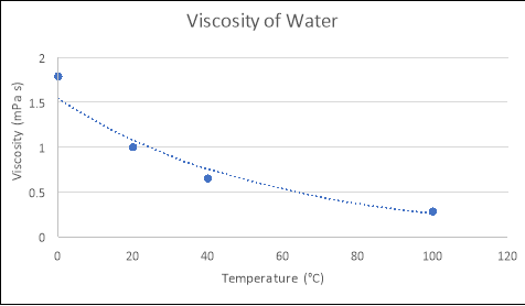
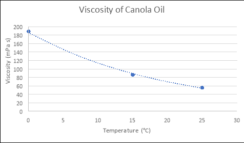
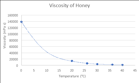
From using the known viscosities of fluids at various temperatures, and developing functions that model these relationships in programs such as Microsoft Excel or on a graphics calculator, the approximate viscosity of a liquid at any temperature can be found by substituting values for temperature into the relevant formula. An example of this process is seen below:
As seen in Figure 1, the equation that models the relationship between temperature and viscosity of water is y = 1.5396e-0.018x. If the temperature of the water was 4ᵒC….
y = 1.5396e-0.018x
y = 1.5396e-0.018 x 4
 y = 1.433 mPas
Therefore, the viscosity of the water at 4áµ’C is 1.433 mPas.
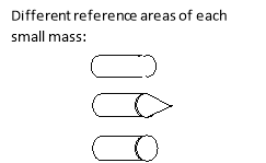
Viscosity is also what causes an object to slow as it travels through a fluid, and is one component in the phenomenon of drag force, ‘the retarding force that acts opposite to the direction of motion of a body or object‘. The drag force of any object is dependent on the viscosity of the fluid it travels through, velocity of the object, reference area of the object, and the drag coefficient.

The following formula can be used to calculate the total drag force acting upon an object (Wikipedia, 2017):

Where:  = Drag force (N),
  = Mass density of fluid (mPas),
  = Flow speed of object relative to fluid (ms-1),
  = Drag coefficient (no units), A = Reference area (m2)
A worked example of this calculation with assumed and exact values is modelled below:
Assume that for a flat surfaced mass travelling through water at 4ᵒC….
 mPas
mPas
= 0.3ms-1
 0.82
0.82
A = 2.5 x 10⁻⁴
The values are then substituted into the drag force formula……
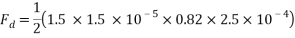
Therefore the drag force of the mass travelling through water at 4áµ’C is approximately 4.6125 x 10⁻⁵N.
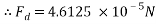
 One component of this force, as represented by in the drag force equation, is a drag coefficient (The Free Dictionary, 2017). As stated in ‘The Physics of Sailing’ by Ryan M. Wilson (2010), ‘intuitively, the drag should depend linearly on the density of the fluid in which the body is immersed (because force depends linearly on mass) and linearly on the area of the body that is exposed to the flow because the volume of fluid that must be displaced as the body moves through it is proportional to this area‘. A range of calculated drag coefficients for various shapes can be seen in Figure 3. It can therefore be concluded that the lower the drag coefficient of an object, the lower the amount of drag force that occurs as it travels through a fluid (Brock University, 2017).
As seen in Figure 2, the drag coefficient of an object is reliant on its shape. It can be concluded that a mass with a flat reference area will travel almost two times slower than that with a spherical reference area. A conical reference area will cause an object to fall slightly slower than a spherical mass, but faster than one with a flat reference area. Theoretically, as deducted from Figure 2, it is concluded that a mass with a spherical reference area will travel faster than one with either a conical and flat surfaced reference area, the latter of these theoretically having the slowest time of fall through a liquid out of the three.
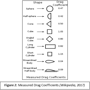
Although many different fields of study incorporate knowledge of drag forces and viscosity, arguably one of the most important applications is found within the engineering of ships and the design of the hulls, specifically in relation to sailing competitions such as the America’s Cup. As one of the largest sailing races in the world, this competition has strict guidelines for ship design, consequently meaning that vessel engineers must ‘find the best combinations (of measurements) to create the fastest ship possible’ (Krepal, 2014). When building, engineers must be familiar with the environmental sailing conditions of the race in order to build the most suitable hull with the least amount of drag – this is determined in regards to the temperature of the sea and its viscosity. As calculating viscosity is a complex procedure, ship engineers often refer to data such as seen in Figure 2 to determine aspects of ship design.

In regards to the speed of the ship, it can be concluded from previous knowledge on drag force that the lower the drag coefficient of a vessel, the easier it is for it to break through the water, overcoming shear force and resulting in a faster travelling time (Krepal, 2014). When unknown, the drag force formula can be rearranged to find the drag coefficient; however, often these values are computed from graphical designs of the ship as the phenomenon of drag force is dependent on many variables. Testing on model ships is also performed to determine how vessels will travel under different conditions (Mecaflux, 2013).
HYPOTHESIS
Based on the previous research, the hypothesis for this experiment is that:
‘If a body is falling in a liquid, then i) the lower the viscosity of the liquid, which decreases as temperature increases, the faster will be the rate of fall of the object, and ii) the lower the drag coefficient of the body, the smaller its drag force will be, as the velocity of an object as it travels through a fluid is inversely proportional to the amount of resistance it encounters.
METHOD
The supplies needed – 1L glass measuring cylinder, 2L water, 2kg honey, 2L canola oil, 3 x 53g cylindrical masses with different reference areas of the same 0.9cm radius (flat, spherical, streamlined/conical), a Thermomix, thermometer, a logbook and pencil, and a video recording device. All measurements and data were to be collected and stored in a logbook and on the video recording device. A risk assessment form was completed before the commencement of the experiment, in order to recognise any potential hazards regarding the equipment that was to be used. It was identified that any device used to heat up the liquids, and the hot liquids themselves, had potential to burn the person completing the experiment, and it was possible for the glass cylinder to topple over and shatter as it was filled with each liquid. Covered shoes were worn during the experimental procedures to protect the feet from any falling objects and glass, and care was taken when using heating devices and handling hot liquids.
As the hypothesis was written in two parts, there were two variables that remained constant depending on the experimental procedure (independent variables) – the first was the temperature/viscosity of each liquid, and the second was the reference area of the masses travelling through each. The dependent variable in both was the velocity of the object.


The equipment was set up for the experiment as depicted in Figure 6. 1L of each liquid was placed in the fridge and cooled to 5áµ’C. 1L of the first liquid, water, was heated in the Thermomix to 37áµ’C and then poured into the glass cylinder. The flat ended mass was dropped from the 1L mark, and its fall was timed and recorded on the video recording device. The object was then extracted from the bottom of the cylinder, and this process was repeated two more times. The flat ended mass was then removed, and the same procedure was performed again for both the spherical and conical shaped masses. After these tests were completed, the water was poured back into the Thermomix and was heated to 50áµ’C. Once at temperature, the water was again poured into the cylinder, and the previously stated processes were repeated for each mass. After these tests were completed, the water was poured into the Thermomix. The chilled water from the fridge was then taken out, checked with a thermometer to be at 4áµ’C, and poured into the cylinder for testing. The previously stated processes for each mass were repeated. After all of the masses had been dropped into the water at all three temperatures, the water was disposed of, and the experimental space cleaned up to prepare for the next round of testing. All results were recorded into various tables in the logbook, and later graphed for analysis.
The second liquid, canola oil, was heated in the Thermomix to 35áµ’C and then poured into the glass cylinder. The previously stated procedures were repeated. All results were recorded into a table, and later graphed for analysis.
The third liquid, honey, was heated in the Thermomix to 35áµ’C and then poured into the glass cylinder. The previously stated procedure was repeated. All results were recorded into a table, and later graphed for analysis.
In this experiment, it is noted that apart from that which were independent and dependant, all other variables were controlled, consequently meaning that every aspect of the testing remained consistent. These controlled variables included the positioning of the glass cylinder and video recording device, the dropping point of the masses, the weight of the small masses used, the radius of the masses, the distance each mass fell, the type of oil and honey used, etc. By controlling all other variables, the results recorded from the testing become more accurate.
RESULTS
(HYPOTHESIS – PART 1)
CALCULATED VALUES FOR VISCOSITY
By using the formulas generated from the Excel graphs in Figure 1, which model the relationships between the viscosity and temperature of each liquid, and substituting in the experimental temperatures for ‘x’ (4, 37 and 50), the empirical viscosities of each fluid at different temperatures were calculated. The tables and graphs of these results follow, with all calculations performed recorded in the logbooks.
WATER
|
Temperature (áµ’C) |
Viscosity (mPas) |
|
4 |
1.433 |
|
37 |
0.791 |
|
50 |
0.626 |
y = 1.5396e-0.018x
CANOLA OIL
y = 186.16e-0.049x
|
Temperature (áµ’C) |
Viscosity (mPas) |
|
4 |
153.026 |
|
37 |
30.375 |
|
50 |
16.064 |
HONEY
y = 138468e-0.117x
|
Temperature (áµ’C) |
Viscosity (mPas) |
|
4 |
86716.073 |
|
37 |
1825.108 |
|
50 |
398.774 |


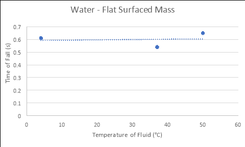
Water
Flat Surfaced Mass
|
Temperature of Fluid (áµ’C) |
Time 1 (s) |
Time 2 (s) |
Time 3 (s) |
Average Time of Fall (s) |
|
4 |
0.41 |
0.62 |
0.81 |
0.61 |
|
37 |
0.62 |
0.50 |
0.50 |
0.54 |
|
50 |
0.66 |
0.60 |
0.69 |
0.65 |


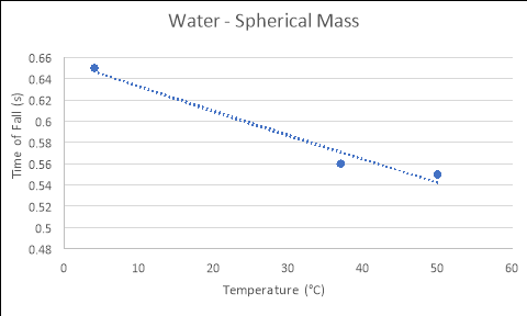
Spherical Mass
|
Temperature of Fluid (áµ’C) |
Time 1 (s) |
Time 2 (s) |
Time 3 (s) |
Average Time of Fall (s) |
|
4 |
0.91 |
0.68 |
0.37 |
0.65 |
|
37 |
0.53 |
0.59 |
0.55 |
0.56 |
|
50 |
0.43 |
0.62 |
0.60 |
0.55 |


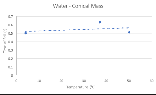
Conical Mass
|
Temperature of Fluid (áµ’C) |
Time 1 (s) |
Time 2 (s) |
Time 3 (s) |
Average Time of Fall (s) |
|
4 |
0.40 |
0.57 |
0.54 |
0.50 |
|
37 |
0.78 |
0.50 |
0.62 |
0.63 |
|
50 |
0.59 |
0.50 |
0.43 |
0.51 |


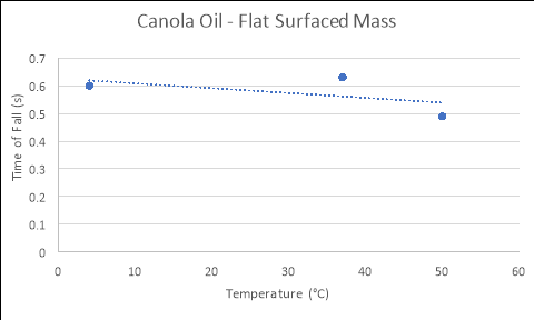
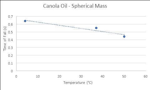
Canola Oil
|
Temperature of Fluid (áµ’C) |
Time 1 (s) |
Time 2 (s) |
Time 3 (s) |
Average Time of Fall (s) |
|
4 |
0.60 |
0.55 |
0.65 |
0.60 |
|
37 |
0.62 |
0.69 |
0.58 |
0.63 |
|
50 |
0.49 |
0.52 |
0.46 |
0.49 |
Flat Surfaced Mass


Spherical Mass
|
Temperature of Fluid (áµ’C) |
Time 1 (s) |
Time 2 (s) |
Time 3 (s) |
Average Rate of Fall (s) |
|
4 |
0.63 |
0.59 |
0.69 |
0.636667 |
|
37 |
0.56 |
0.56 |
0.53 |
0.55 |
|
50 |
0.45 |
0.46 |
0.42 |
0.443333 |


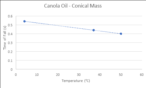
Conical Mass
|
Temperature of Fluid (áµ’C) |
Time 1 (s) |
Time 2 (s) |
Time 3 (s) |
Average Rate of Fall (s) |
|
4 |
0.67 |
0.53 |
0.43 |
0.543333 |
|
37 |
0.46 |
0.49 |
0.38 |
0.443333 |
|
50 |
0.36 |
0.45 |
0.39 |
0.4 |


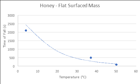
Honey
Flat Surfaced Mass
|
Temperature of Fluid (áµ’C) |
Time 1 (s) |
Time 2 (s) |
Time 3 (s) |
Average Rate of Fall (s) |
|
4 |
2040 |
2257.2 |
2008.2 |
2101.8 |
|
37 |
498.6 |
489 |
508.2 |
498.6 |
|
50 |
84 |
91.2 |
95.4 |
90.2 |


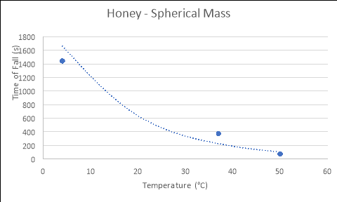
Spherical Mass
|
Temperature of Fluid (áµ’C) |
Time 1 (s) |
Time 2 (s) |
Time 3 (s) |
Average Rate of Fall (s) |
|
4 |
1428 |
1537.2 |
1362.6 |
1442.6 |
|
37 |
362.4 |
370.2 |
389.4 |
374 |
|
50 |
72 |
70.8 |
73.8 |
72.2 |


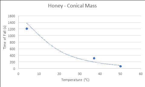
Conical Mass
|
Temperature of Fluid (áµ’C) |
Time 1 (s) |
Time 2 (s) |
Time 3 (s) |
Average Rate of Fall (s) |
|
4 |
1188 |
1135.2 |
1305 |
1209.4 |
|
37 |
307.2 |
305.4 |
320.4 |
311 |
|
50 |
66.6 |
65.4 |
67.2 |
66.4 |


HYPOTHESIS – PART 2
CALCULATED DRAG FORCES
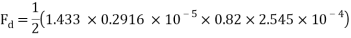
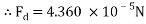
Worked Example:
Flat surfaced mass travelling through water at 4°C
 mPas
mPas
 = 0.2916 ms-1
 0.82
0.82
A = 2.545 x 10⁻⁴
The values are then substituted into the drag force formula……

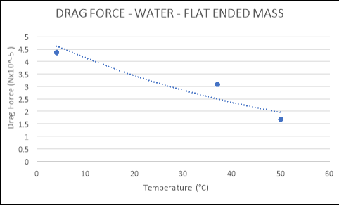
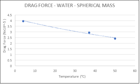
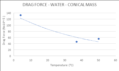
WATER:
|
TEMPERATURE (°C) |
DRAG FORCE (Nx10-5) |
|
Flat |
|
|
4 |
4.3600 |
|
37 |
3.0830 |
|
50 |
1.6840 |
|
Spherical |
|
|
4 |
3.9480 |
|
37 |
2.9358 |
|
50 |
2.4084 |
|
Conical |
|
|
4 |
132.3700 |
|
37 |
46.0270 |
|
50 |
55.5820 |
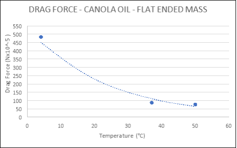
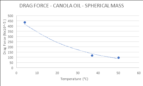
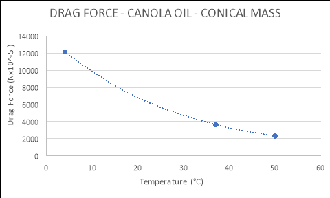
CANOLA OIL:
|
TEMPERATURE (°C) |
DRAG FORCE (Nx10-5) |
|
Flat |
|
|
4 |
483.020 |
|
37 |
86.971 |
|
50 |
76.033 |
|
Spherical |
|
|
4 |
434.850 |
|
37 |
116.860 |
|
50 |
96.567 |
|
Conical |
|
|
4 |
12120.000 |
|
37 |
3620.000 |
|
50 |
2320.000 |


HONEY:
|
TEMPERATURE (°C) |
DRAG FORCE (Nx10-5) |
|
Flat |
|
|
4 |
0.0223060 |
|
37 |
0.0083423 |
|
50 |
0.0556950 |
|
Spherical |
|
|
4 |
0.0485340 |
|
37 |
0.0151850 |
Cite This Work
To export a reference to this article please select a referencing stye below:
Related Services
View all


DMCA / Removal Request
If you are the original writer of this essay and no longer wish to have your work published on UKEssays.com then please click the following link to email our support team:
Request essay removal