Remote Sensing Bathymetry of Coral Reefs
| ✅ Paper Type: Free Essay | ✅ Subject: Environmental Studies |
| ✅ Wordcount: 3194 words | ✅ Published: 04 Sep 2017 |
Remote Sensing Bathymetry of Coral Reefs Based on the Spatial Relationship between Different Depths
Rongyong Huang1, 2, 3, Kefu Yu1, 2, 3*, Yinghui Wang1, 2, 3, Jikun Wang1, 2, 3, Lin Mu4, Wenhuan Wang1, 2, 3
1 Coral Reef Research Centre of China, Guangxi University, Nanning, China
2 Guangxi Laboratory on the Study of Coral Reefs in the South China Sea, Guangxi University, Nanning, China
3 School of Marine Sciences, Guangxi University, Nanning, China
4 Institute of Complexity Science and Big Data Technology, Guangxi University, Nanning, China
Abstract:
Shallow water depth inversion using multispectral images is fundamentally important for marine surveying and mapping over large areas or in remote locations and especially for research on coral reef ecosystems. However, most recent studies on water depth estimation have focused on the construction, verification, and application of water depth inversion models. We compared several kinds of n-band combination models and their extensions and found that only limited improvements to their performance can be made by modifying the model expressions. Therefore, we propose a novel adjustment method to globally refine estimations of the water depths[j1] of coral reefs by employing an optimization approach. The objective function is mainly constructed using the weak dependences of each pair of neighbouring pixels and the implicit constraints of the sea-land interface pixels. The experimental results from ZY-3[j2] multispectral imagery of Weizhou Island demonstrate that the method is effective at improving the accuracy of depth estimates. In addition, the analysis shows that the results are affected less by the models’ expressions when the proposed method is used. Accordingly, we suggest modifying common n-band combination models with our method to obtain a higher level of accuracy.
Keywords: Water Depth, Coral Reef, Multispectral Imagery, Bands Combination, Refinement, Optimization
1 Introduction
Accurate bathymetric measurements over large areas or in remote locations are considered to be fundamentally important in monitoring the sea bottom and for producing nautical charts for marine navigation (Papadopoulou et al., 2015; Stumpf et al., 2003; Su et al., 2008). These measurements are directly relevant to environmental management, exploration, defence and research applications (Brando et al., 2009). For example, coral reefs strongly influence the physical structure of their environment due to their natural development. The associated water depth information is fundamental for discriminating and characterizing coral reef habitats, such as patch reefs, the spur-and-groove system around the reef front, and sea grass beds (Stumpf et al., 2003). Knowledge of the water depth also facilitates estimations of the bottom albedo, which can improve habitat mapping (Mumby and Clark, 1998). Therefore, shallow water depth measurements have always been an important component of marine surveying and mapping.
However, until recently, bathymetric surveying of shallow sea water has mainly been dependent on conventional ship-borne echo sounding operations. This technique is expensive and time-consuming, particularly in shallow water areas where dense networks of measurement points are required (Papadopoulou et al., 2015). In addition, it is difficult to measure the water depth in remote and dangerous areas, where massive hidden reefs can make them unreachable.
For this reason, we focus on enhancing the remote sensing data-based solutions that have been proposed over the past few decades to increase their cost- and time-effective characteristics and improve their performance. One motivation is to provide bathymetric results to assist in research on the effects of ambient environmental conditions on the coral reef of Weizhou Island. In addition, we expect to improve the remote sensing data-based solutions for multispectral images to attain relatively accurate and reliable water depth estimations that may be applied to remote, large, or dangerous areas in the future.
Based on the law that light is attenuated exponentially with depth in the water column, Lyzenga (1978, 1985) showed that using two bands could correct the errors that result from different bottom types provided that the ratio of the bottom reflectances between the two bands for all bottom types is constant over the scene. Thereafter, Lyzenga (1978, 1981, 1985) and Lyzenga et al. (2006) attempted to derive the water depth using a linear transformation of pure rotation to construct an index that is only dependent on the water depth and further proposed two band and n-band combination models for water property-independent and bottom reflectance-independent water depth extraction. Doxani et al. (2012) further evaluated the effectiveness of the high spatial and spectral resolutions of Worldview-2 imagery for water depth measurements using Lyzenga’s linear bathymetry model. Based on the same exponential model, Clark et al. (1987) introduced a linear multiband method for shallow water extraction, which was tested using bands 1 and 2 of Landsat TM imagery from the vicinity of Isla de Vieques. Stumpf et al. (2003) further improved the linear multiband method to an empirical solution over variable bottom types using a ratio of reflectances with only two tunable parameters.

Assuming that the water quality and bottom substratum are homogeneous, Bierwirth (1993) outlined a method that unmixed the exponential influence of depth in each pixel by employing a mathematical constraint, which had previously been applied in the analysis of Landsat TM data from Hamelin Pool in Shark Bay, Western Australia. Lafon et al. (2002) proposed a semi-empirical bathymetric methodology based on the Hydrolight radiative transfer code calibrated with in situ bottom reflectance and effective attenuation coefficient measurements and applied it to determine the depth from SPOT images and develop topographic maps of the tidal inlet of Arcachon. In contrast, Sandidge and Holyer (1998) empirically employed a neural network as a paradigm for mapping spectral radiance curves for water depths in the presence of variable bottom reflectance and water attenuation characteristics.
Lee et al. (2001, 1998, 1999) developed a semi-analytical model for shallow water remote sensing based on the analytical model proposed by Maritorena et al. (1994) and then used an inversion-optimization approach to simultaneously derive water depth and water column properties from hyperspectral data in coastal waters based on the proposed model. Brando et al. (2009) further enhanced the physics-based inversion/optimization approach that was developed by Lee et al. (2001, 1998, 1999) by considering the concentrations of optically active constituents in the water column, different types of substratum cover, and the contribution of every substratum to the remote sensing signal, which was then successfully applied to airborne hyperspectral data from Moreton Bay, Australia.
Although they did not address the problem completely, these studies laid the foundation for the further development of water depth inversion. Many recent studies have focused on improvements, comparisons, and applications of these models. Papadopoulou et al. (2015) used Lyzenga’s linear bathymetry model (Lyzenga, 1978; Lyzenga et al., 2006) and high resolution IKONOS-2 imagery to create digital bathymetric maps of the coastal area of Nea Michaniona, Thessaloniki, in northern Greece. Yuzugullu and Aksoy (2014) compared the linear regression model with an empirical non-linear regression model to predict the depths in Lake Eymir based on WorldView-2 multispectral satellite images, and the results showed that the non-linear regression model predicted the depths slightly better than the linear model. Gholamalifard et al. (2013) tested the single band algorithm (SBA), the principal component analysis (PCA) method, and the multi-layer perceptron neural network between visible bands and one output neuron (MLP-ANNs) method for bathymetry and found that MLP-ANNs produced the best depth estimates. Rasheed et al. (2013) also compared the SBA and PCA bathymetric models from satellite imagery in the Southern Caspian Sea and concluded that PCA matched the control points slightly better than SBA. Mohamed et al. (2016) improved the linear multiband method by using the Ensemble Learning (EL) fitting algorithm of Least Squares Boosting (LSB) to develop bathymetric maps in shallow lakes from high resolution satellite images and water depth measurement samples using Eco-sounder; they obtained better performance and accuracy than the conventional PCA and generalized linear models. Additional related studies include Jawak and Luis (2016), Su et al. (2008, 2015), Smith et al. (2013), Lee et al. (2011), and Monteys et al. (2015).
We reviewed several related studies on obtaining bathymetry from multispectral imagery over the last several decades and found that several effective water depth inversion methods have been developed and applied. Most of these methods prioritized the construction, verification, and application of water depth inversion models. They aimed to map each individual pixel to one water depth and ignored the weak dependences between one pixel and its neighbourhoods and the implicit constraints of the sea-land interface pixels. Therefore, we focus on using two such constraints, that the water depths of every pixel and its neighbourhood should be as similar as possible to each other and that the water depths of the sea-land interface should be approximately zero, to refine the water depths that are derived from the two band and n-band combination models of Lyzenga (1978, 1981, 1985), Lyzenga et al. (2006), Stumpf et al. (2003), and Papadopoulou et al. (2015).
Specifically, our first main goal is to compare the different kinds of n-band combination water depth inversion models to test their performances. A novel adjustment method is then proposed to refine the water depths that are estimated by these models based on the two conditions described previously and an optimization approach. Finally, the effectiveness of the method is verified using ZY-3 multispectral imagery of Weizhou Island, and a water depth inversion approach is then suggested that combines an n-band combination model with the proposed refinement approach based on the experimental results. Details about the methods are presented in the following sections.
2 Materials and Preprocessing
2.1 Study Area
The study area is Weizhou Island in the Beibu Gulf, northern South China Sea. As shown in Fig. 1, Weizhou Island is oval and is located at 21°00´-21°05´ N, 109°00´-109°10´ E, which is approximately 36 miles from Beihai, Guangxi. Although the seawater transparency varies from 3.0 m to 10.0 m, Weizhou Island is ideal for coral growth due to the annual average sea surface temperature and salinity of approximately 24.55 ℃ and 31.9‰, respectively. Coral reefs have developed around Weizhou Island since the mid-Holocene, and the reefs cover an area of approximately 6-8 km2 (Yu, 2012; Yu and Zhao, 2009). These coral reefs have long been a focus of studies on the response of coral to global warming and human disturbances because they are in a relatively high latitude area and are heavily influenced by anthropogenic activities (Yu and Zhao, 2009).
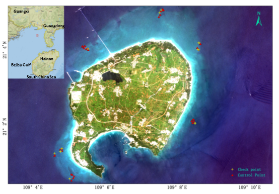
Fig. 1. True Colour Imagery (ZY-3) of Weizhou Island and Experimental Control/Check Points for Water Depth Estimation
2.2 Experimental Data and Preprocessing
The ZY-3 satellite was launched on January 9, 2012, as the first civil high-resolution optical transmission surveying and mapping satellite of China. It is equipped with four optical cameras, including a nadir panchromatic Time Delay and Integration (TDI) CCD camera with a ground resolution of 2.1 m, two back/forward sight panchromatic TDI CCD cameras with a ground resolution of 3.6 m, and a nadir multispectral camera with a ground resolution of 5.8 m. A ZY-3 multispectral image that was acquired on August 24, 2015, was chosen as the remote sensing source data for our experiments. The positioning information of the satellite was assigned to the imagery using the World Geodetic System (WGS84). Additional band information is presented in Tab. 1.
Tab. 1. Band Information of the ZY-3 Multispectral Satellite Imagery
|
Bands |
Wavelength (nm) |
Radiometric Calibration Coefficients ( |
|
|
Gain |
Offset |
||
|
Blue |
450-520 |
0.233 |
0 |
|
Green |
520-590 |
0.2162 |
0 |
|
Red |
630-690 |
0.1789 |
0 |
|
Near-Infrared |
770-890 |
0.1949 |
0 |
 )
)Before the water depth estimation is performed, the main preprocessing steps of the multispectral imagery can be summarized as follows.
1) Radiometric calibration: radiometric calibration was performed to transform the digital numbers (DN) to planet radiance using the radiometric calibration coefficients shown in Tab. 1.
2) Atmospheric correction: atmospheric correction is performed to remove the effects of the atmosphere on the reflectance values of images taken by a satellite or airborne sensors. In this paper, atmospheric correction was specifically used to correct the planet radiance to remote sensing reflectance. This was done using the FLAASH module of ENVI 5.1 based on Moderate Resolution Transmission (MODTRAN).
We also measured 31 control points and 13 check points in the field during May 2015 for the construction and assessment of the water depth inversion models (Fig. 1). The water depths were measured by a SM-5A hand-held portable depth sounder with an accuracy of 0.1 m, and the horizontal positions were mapped with a Magellan eXplorist 610 hand-held GPS navigation instrument with an accuracy of 3-5 m. This accuracy satisfies the application of the ZY-3 multispectral imagery, which has a resolution of 5.8 m. The in situ measurements can be matched to the satellite data by applying the positioning information of the imagery.
Finally, we need to eliminate the influence of the different tidal levels because the in-situ measurements and the imagery were collected at different times. We selected the tide level in the imagery as a reference and then corrected the in-situ measured water depths to the reference level.
3 Methodology
3.1 Principle of Water Depth Estimation
This section presents the details of light propagation in the water column as the theoretical basis for water depth inversion models and the water depth inversion model patterns that will be compared in the following experiments.
3.1.1 Light Propagation Model in the Water Column
The light that is received by a satellite is affected by both the atmosphere and the water column (Fig. 2). However, because the effects of the atmosphere on the reflectance values of the images have already been removed by the atmospheric correction in the preprocessing, we focus on the effects of the water column in the following water depth estimation.

Fig. 2. Light Propagation in the Water Column
As shown in Fig. 2, light entering a water column is subjected to absorption and scattering by both the water body and the substrate. According to the Beer-Lambert Law, the attenuation of light energy decreases exponentially with the water depth ( ) and may be described as follows (Bierwirth, 1993; Zoffoli et al., 2014):
 (1)
(1)
where  is the water-leaving radiance in the presence of the bottom,
  is the radiance reflected by the substrate material for no water cover (i.e.,
  ),
),  is the water-leaving radiance for an infinitely deep water, and
  is the effective attenuation coefficient for the water column.
Because the reflectance is proportional to the radiance, Eq. (1) can be normalized to reflectance as follows:
 (2)
(2)
i.e.,
 (3)
(3)
For any two bands  and
and  , taking their ratio gives:
 (4)
(4)
Taking the logarithm of both sides of Eq. (4) gives:
 (5)
(5)
i.e.,
 (6)
(6)
In general, the bottom reflectances and the water attenuation coefficients are clearly different due to the variations of the bottom types and the water qualities, but many previous studies have shown that both the ratio of the bottom reflectances (i.e., ) and the difference between the water attenuation coefficients (i.e.,
  ) of a pair of wavelength bands remain relatively constant in a given scene (Lyzenga, 1978; Paredes and Spero, 1983). In other words, the water depth may usually be modelled as:
 (7)
(7)
where  ,
,  , and
, and  . The coefficients
  and
and  are regarded as constants that can be determined by linear regression of the water depths measured in situ.
3.1.2 Water Depth Inversion Models
Except for the form described by Eq. (7), most of the patterns that are considered in our comparison fall in the following two categories.
1) Band combination models (Lyzenga, 1978, 1981, 1985; Lyzenga et al., 2006; Papadopoulou et al., 2015; Stumpf et al., 2003) with the following form:
 (8)
(8)
Linear relationships of different items must be carefully considered in the form of Eq. (8). For example, there is a linear relationship between the first three bands (blue, green, and red) of ZY-3 multispectral imagery as follows:
 (9)
(9)
Hence, we cannot select  ,
,  , and
, and  as the independent variables of Eq. (8) at the same time.
To more conveniently eliminate such linear relationships, we further regard the following identical equations when multispectral bands are used:
 (10)
(10)
where  , and
, and  .
.
Substituting Eq. (10) into Eq. (8) gives another form of band combination models:
 (11)
(11)
Similar to Eq. (7), we can determine the coefficients of Eq. (8) and Eq. (11) via linear regression and the in situ measured water depths.
2) Rational function models with the following forms:
 (12)
(12)
or
 (13)
(13)
where
 (14)
(14)
 (15)
(15)
Rational function models may be regarded as empirical extensions of the band combination models. We can solve  and
and  as follows: traverse all
  and
and  that satisfy Eq. (14) and Eq. (15) with a certain step (i.e., 0.02 in our experiments), estimate each
  and
and  of
of  and
and  via linear regression, and then choose the values of
  ,
,  ,
,  , and
, and  that give the maximum R-squared value as the optimal coefficients of the water depth estimation model.
3.1.3 Estimation of Deep Water Reflectance
In addition to the band combination patterns presented above, we also consider several patterns that are constructed using different deep water reflectance values; i.e., we use of the following three methods to assign different values to the deep water reflectance  in the comparison:
1) Ignore the influence of ; i.e.,  ;
;
2) Assign the minimum water reflectance to  ; i.e.,
  .
.
3) For a certain model (e.g., Eq. (7), Eq. (8), or Eq. (11)), we traverse all  in
in and find the value that provides the model’s maximum R-squared value. This
  is called the optimal deep water reflectance; in contrast,
  or
or  is then called the simple deep water reflectance.
Note that if the latter method is used for the assignment, different models will usually be assigned to different values of  .
.
3.2 Refinement of the Estimated Water Depths
As discussed in Section 1, we further make use of the two conditions (i.e., the weak dependences between one pixel and its neighbourhoods and the implicit constraint conditions of the sea-land interface pixels) to refine the water depths that are estimated by the models presented above after the comparison is finished. The details are as follows.
3.2.1 Model for Refining the Water Depths
Assume that the multispectral imagery  is composed of
  pixels and that each pixel of
  has the form of:
 The corresponding water depth was estimated using one of the models presented above, and this water depth was denoted by
  .
.
According to the weak dependences in neighbourhoods, for any pixel  and one in its neighbourhood
 , their corresponding water depths, which are denoted as the unknowns
  and
and  , respectively, should be as close to each other as possible; i.e.,
 (16)
(16)
Another condition that can be used to refine the water depths is that the water depths of the sea-land interface should be as close as possible to zero; thus, for any pixel  of the sea-land interface, we have:
 (17)
(17)
For an integrated consideration of Eq. (16) and Eq. (17) and to ensure that the water depth  is not significantly different from
  for any pixel
  , we can construct an objective function (Eq. (18)), and all unknown
  can then be solved by minimizing the objective function:
 (18)
(18)
where  ,
,  ,
,  , and
, and  are the corresponding weights of each term of the objective function. If pixel
  is located in an effective region, then
 ; otherwise,
  . If pixel
  and its neighbourhood
  are both located in an effective water region, then
  ; otherwise,
  . If pixel
  is a sea-land interface pixel, then
  ; otherwise,
  . The parameters
  and
and  represent the strengths of these two constraint conditions, where their values are defined by the actual conditions. For example, we take
  and
and  in the experiments in this paper.
Note that the purpose of introducing  to the objective function is to simplify the calculation; if and only if pixel
  is an invalid pixel (e.g., a pixel that is located on the island without water), then
  ,
,  , and
, and  . Thus, all of the values of the invalid pixels must be 0 to minimize the objective. This means that we can distinguish and label the effective water pixels before the optimization but do not need to distinguish between the effective water pixels and the invalid pixels in the optimization approach.
3.2.2 Solution of the Refinement Model
According to the least squares method, we need to solve Eq. (19) to minimize the objective function:
 (19)
(19)
i.e.,
 (20)
(20)
There are so many unknowns ( ) in Eq. (19) and Eq. (20) that it is difficult to solve the equations directly. Fortunately, we can instead employ the Jacobi iteration method to solve these linear equations using the following iterative formula:
 (21)
(21)
where
Cite This Work
To export a reference to this article please select a referencing stye below:
Related Services
View all


DMCA / Removal Request
If you are the original writer of this essay and no longer wish to have your work published on UKEssays.com then please click the following link to email our support team:
Request essay removal