Population and Community Ecology Estimation Study

Population and Community Ecology

Intro:

Population ecology is the objects of study of which are the change in the number of populations, the relationship of groups within them. Within the framework of population ecology, the conditions under which populations are formed are being ascertained. It describes fluctuations in the numbers of different species under the influence of environmental factors and establishes their causes. The main factors that effect on the size of population are density, abundance and distribution (Friedl, 2019).

In this experiment were used few methods to estimate the population of the species: Removal method and Mark-Recapture method.

Removal Method:

This method is very convenient for estimating the number of small organisms, especially insects, on a certain part of the meadow or in a certain volume of water. With a wave of a special grid, animals are caught, the number of caught is recorded and not released until the end of the study. Then the capture is repeated three times, with each time the number of animals caught decreases. When plotting, the number of animals caught at each catch is noted against the total number of animals caught earlier.

Mark-Recapture technique:

This method involves trapping an animal, marking it in such a way as not to harm it, and releasing it where it was caught, so that it can continue normal livelihoods in the population. For example, gill covers of nets caught by fish are attached to aluminium plates, or rings are put on the legs of nets caught by nets. Small mammals can be marked with a paint, incise the ear or cut off the fingers, arthropods are also marked with paint. In any of the cases, a form of coding can be applied that allows one to distinguish individual organisms. The captured animals are counted, a representative sample of them is tagged, and then all animals are released to the same place. After some time, the animals are again caught and the number of animals with a label is counted in the sample (khanacademy.org, 2019).

The population size was estimated by using the following two formulas:

Number 1:

 n= number in sample 2

 m= number marked (McCarthy, 2019)

Method:

For population size estimation were performed two experiments.

In the first experiment (Mark-Recapture method) were used jelly beans. And for Removal method were used white beans and the brown beans instead of pinto beans.

Results:

 Table 1. Recorded data of Marked-Recaptured technique.

N= population estimate

 M= total marked

 n= number in sample 2

 m= number marked

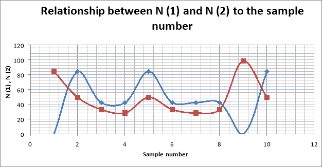
Figure 1. The graph is showing the relationship between two population estimates to the sample number. Blue colour represented N (1) and Red represented N(2).

 Table 2. Showing assumption of Mark-Release-Recapture.

N= population estimate

 M= total marked

 n= number in sample 2

 m= number marked

 Table 3. Showing data results for Removal Method data.

Table 4. Showing data gained from Predator-Prey Simulator.

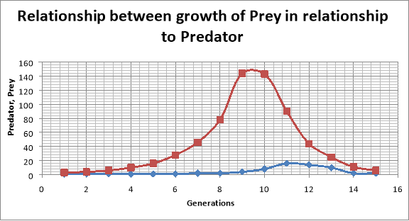
Figure 2. The graph showing the relationship between the growth of Prey in relation to Predator. Red colour represented Prey and Blue represented Predator.

Discussion:

For Mark-Recapture method (Table 1, Figure 1) were used two formulas. Formula Number one: N (1) and formula Number two N (2) respectively. Despite that results from both formulas were close enough to each other, but it was considered that the results from formula N (2) were more accurate and closer to the real actual number of population. This happened because N (2) in this formula you are adding “+1”, which preventing calculation from negative numbers or zero.

In removal method (Table 3) most of the sampling efforts were consistent: 6 times were the same numbers, and the rest trials were biased for +/- 1, 2 or 3. This means that the population estimate would not be highly biased.

 In Prey and Predator simulation as time goes by the relationship of both species will be more or less proportional. This means that both species controls population of each other. For example if population of prey increases, so that mean during few generations the population of predator will increase. After few generations the population of prey will decrease and that will decrease population of predators as well.

If new predator would be added to the system, it will negatively affect on prey population. Of course that will depend from prey population. If there are more predators than prey, there will be possibility for prey to disappear or minimize its population. And that will lead to decrease of population of predators as well. This means that every increase of predator population after slight lag will decrease population of prey.

The Prey-Predator simulation represents animals population cycle during the time periods and generations. It models the dynamics of prey and predator in the nature.

References:

• Friedl, S., (2019). Population Ecology: Definition, Theory & Model [online] Available from; https://study.com/academy/lesson/population-ecology-definition-theory-model.html {accessed on 14 Feb 2019}
• khanacademy.org (2019).  Population size, density, & dispersal [online] Available from; https://www.khanacademy.org/science/high-school-biology/hs-ecology/hs-population-ecology/a/population-size-density-and-dispersal {accessed on 14 Feb 2019}
• McCarthy S., (2019). 2^nd Year Applied Ecology Practical Manual. Dudalk: DKIT