Importance of Frequency Determination Through Fast Fourier Transform Graphical Analysis
| ✅ Paper Type: Free Essay | ✅ Subject: Engineering |
| ✅ Wordcount: 3168 words | ✅ Published: 18 May 2020 |
Importance of Frequency Determination Through Fast Fourier Transform Graphical Analysis
1. Introduction:
Determining frequencies of an object is important in engineering. When determining frequencies of any object, it is important to know what represents a good approach to finding this value. In this lab, a guitar was used to determine the frequency of each string using various graphing and filtering techniques. These graphing and filtering techniques ranged from high-pass, low-pass, and bandpass, to simply using the unfiltered and filtered data in a single sided amplitude spectrum graph. These methods of analysis will be discussed in §2. After conducting the guitar experiment, another was preformed but using a test plan that was created based on the knowledge gained from the previous experiment. One of the more important aspects in this lab was the use of sampling rate. This will be discussed in §4 and will link the methods used, and how different frequencies require different methods to determine accurate frequency ranges to determine vibration levels.
2. Methods of Analysis
2.1 Methods of Guitar Frequency Analysis
In the first section of this lab, a guitar was used for a few quick and important experiments to help understand the importance of the Data Acquisition System (DAQ,) and how t can be used in the assistance of determining frequencies. For the first part of the lab, a block code was created using the lab manual as a guide. This code was simple, and allowed for the frequency’s to be eventually found by implementing a accelerometer. An accelerometer uses a piezo-electric substance which is in part a transducer, or the actual accelerometer. This device can be calibrated given the outputting voltage values and then turned into accelerations (Liu 2019.) The sensor was surrounded in a semi sticky substance which was used to adhere to the guitar to receive the input of the string being plucked. The purpose of each string being plucked was so the frequency for each could be determined using sampling rate, and filtering. The sampling rate is vital to show the recordings in a true nature. These recordings could give off an aliased frequency, or a false reading. To ensure this does not happen, the sampling frequency needs to be set at a high enough rate to ensure the aliased frequency is not recorded. This was achieved by using estimated guesses on the sampling rate, and then taking 10% of the determined value to get the sampling frequency. The experiment was conducted by doing each string individually for a given amount of time, and then repeated on each string but with 10 plucks instead of one. This was done to give a more accurate reading of the frequency of the string and to show a common frequency that all 10 plucks would be around. Now that all the data was collected for the single string plucks, and each string plucked 10 times, MATLAB was used to help show graphically how these frequencies were found from the DAQ. The Fast Fourier Transform (FFT) function in MATLAB was given by the instructor to use. It should be noted that depending on which graph was needed to be found, some of them needed to be scripted out by using a (%) to ensure the code would run properly. The graphs that could be found were the unfiltered data, bandpass filter, high-pass filter, and low-pass filter. Before the steps to get these graphs are discussed, the type of filters will be described. Simply put, the high-pass, low-pass, and bandpass filters allow for frequencies that are above, below, and both above and below to be deleted from detection respectively. There are advantages to all three, and these will be discussed in §4. Now that the filters are described, it be noted that the MATLAB function given is needed to get these graphs. One of the most important points to make about the MATLAB code is that the sampling frequency must match that of the chosen frequency in the DAQ to ensure that the x-axis for all the graphs is correctly displayed. This code used represents the summation described below in equation 2.1.1 which shows the mathematical use of FFT.
|
|
2.1.1 |
This is the equation behind the FFT code used in MATLAB. This equation uses the sampling frequency that was described above alongside the data collected by the DAQ which includes the time, to get the single-sided amplitude graphs which will be shown in section (3) (Liu 2019.)

2.2 DAQ Analysis on Varying Motor Sizes and Frequencies
The second phase of the lab was to use a rectangular block with two motors inside, both of different radius propellers, and to place the sensor over the smaller motor and see if the frequency for this motor could be determined. The same MATLAB FFT function was used in a similar way to get the corresponding graphs discussed in §3. To do this, the sensor was placed directly over the location of the smaller motor to ensure the frequency of the motor was included in the measurement. The motors were running for a given amount of time and the data that was collected was implemented into the MATLAB code discussed above. The purpose of this experiment was to use the code to obtain an unfiltered frequency that was designated on the graph as a high spike, showing where the most frequent measurement was. This allowed for a comparison of this frequency, and the corresponding graphs, and the frequencies of equation 2.2.1. Note that three equations are used in this but all three are vital when showing alias error which will be discussed in §4.
|
|
2.2.1 |
 ,
, ,
,
In this equation,  represents the acquired value from the unfiltered graph that was obtained, and
  is the resulting value from the change. These two experiments in sections 2.1.1 and 2.2.1 allowed for a new trial to be ran where a test plan could be created based on the knowledge from these tests.
2.3 Test Plan for Obtaining Cellphone Frequency
The final experiment conducted was using the phone of a lab member and trying to determine the frequency. To do this, a test plan is required to ensure more accurate processes and approaches are used to get a better understanding of this frequency finding method. The first step was to realize that most people have a phone case of some sorts, so it was clever to do this experiment with the cover both on and off. Using a typical scientific method approach, the phone was tested both with and without the case, using different mediums to ensure the frequency being tested was the same. The phone was called by another group member and the program was ran for a few seconds. No time restraint is necessarily needed but one could be used by letting the phone ring for a fixed amount of time to ensure more accurate results. This was done as stated using different mediums, which consisted of placing the phone on the floor, leaving it in someone’s hand, placing it on a table, placing it in a pants pocket, and putting it in a backpack compartment. These mediums were consistent for both the phone with and without the case. To try to ensure the results were as similar as possible, similar placements for the phone were used with the cover on and off. The point of using these steps and doing the measurements with and without a phone cover is to ensure that the frequency is the same through similar mediums, and that the frequency was consistent throughout the experiment, as it was predicated to be. In §3, there will be a chart containing the rank, frequency, and where the phone was located to give a better representation to the values.
2.4 Uncertainty Methods for Guitar
After the experiment was concluded for the guitar, the confidence interval and precision interval were
determined from the data collected for the high E string. This was done using equation 2.4.1 for the confidence interval. Where x bar is the mean of the data, tvp is the value found from the time distribution chart, and Sx is the standard deviation.
|
|
2.4.1 |
The precision interval also needed to be calculated and was done by using equation 2.4.2.
|
|
2.4.2 |
3. Results:
3.1 Results for Guitar Experiment
For the experiments using the guitar, the best representation of the process used would be to show how the frequency of one string looks using the MATLAB code to graph the data. This can be seen in Figure 1, showing a single sided amplitude graph for the high E string of the guitar.
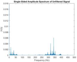
Figure 1. This graph shows the amplitude spectrum of the unfiltered high E string which was plucked 10 times. This was used to ensure a consistent reading would be recorded and based on the highest peak the frequency was determined to be 329 Hz.
Figure 1 gives an average view of what all six graphs for the strings would look like. The only difference is the highest peak would be higher or lower depending on the string.
3.2 Motor Analysis Results
For the second part of the experiment, the motor analysis will be shown graphically using both unfiltered and filtered graphs, along with the three figures corresponding to equation 2.2.1. Figure 2 shows the unfiltered and filtered graphs for the motor.
|
a.
|
b. |
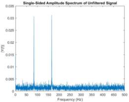
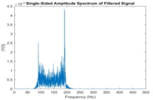
Figure 2. Graph (a) shows the data collected from the motors in a single sided amplitude unfiltered graph. The high and low frequencies were determined to be 170 Hz and 85 Hz and can be seen by the peaks on the graph. Graph (b) shows the filtered version of the same data with a better visual for the same values in graph (a).
After the data collected was graphed and analyzed, the high frequency of 170 Hz was used to get new frequencies based on equation 2.2.1. Figure 3 shows all three new sample frequencies and the corresponding graphs.
|
a. |
b. |
c. |
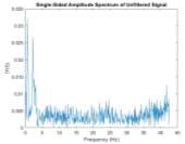
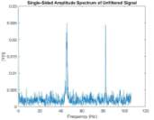
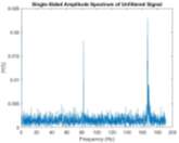
Figure 3. These three graphs show the corresponding  value calculated for 0.5(a), 1.25(b), and 2.25(c). These graphs were unfiltered, only changing the sample frequency for each.
The three graphs above will be explained in detail in §4.
3.3 Cell Phone Test Plan Results
As described in §2.3, the chart with the corresponding value of frequency from the test plan will be shown in Table 1 below. These values were collected using the methods described in the test plan.
|
Position |
Frequency (Hz) |
Rank (1-10) |
|
Hand |
150.6 |
4 |
|
Floor |
150.5 |
2 |
|
Bookbag |
150.5 |
1 |
|
|
150.5 |
3 |
|
Table |
150.2 |
5 |
|
Hand (cover) |
449.3 |
9 |
|
Floor (cover) |
50.54 |
8 |
|
Bookbag (cover) |
150.5 |
7 |
|
Pocket (cover) |
0.000 |
10 |
|
Table (cover) |
148.2 |
6 |
|
Table 1. This chart shows the recorded frequency for all 5 locations with and without the phone cover, then ranks them 1 being the best 10 being the worst. |
||
3.4 Uncertainty Analysis Based on Guitar String Data
For the guitar experiment, the confidence and precision intervals were calculated. This was done using equations 2.4.1, and 2.4.2. These calculations where based on the high E string being plucked 10 times. Table 2 shows the values for both intervals.
|
Confidence Interval (Hz) |
Precision Interval (Hz) |
|
0.00357885 |
0.0307301 |
|
Table 2. This table shows the values for both the confidence interval and precision interval for the high E string being plucked 10 times. |
|
It should be noted that these values are in Hz and are needed for determining how accurate the data can be interpreted as.
4. Discussion:
This lab used repetitive frequency analysis with filtering techniques to help create a valid test plan for a separate experiment. The first part of this lab involved a guitar to record raw data and then use MATLAB to get graphical representation of the unfiltered and filtered values. The most important step in this process was choosing a correct sampling frequency. Sampling frequency is vital because it is not only directly related to the sampling rate but having an incorrect sampling frequency can cause error in the reading. To make sure the sampling frequency is at an appropriate level, the system must be analyzed. For example, the guitar vibrates at a relatively fast rate, so a sampling frequency that is too low will cause error in the readings and give false values for the true frequency at which is vibrating. This shows that a high enough frequency needs to be used to ensure that the string plucked was being read at the correct level. For all experiments in the lab, the sampling rate was simply 10% of the sampling frequency. The sampling rate is vital because it recorded an amount of measurements based on a amount of time. On the other hand, a sampling frequency that is set too high will cause more error in the reading due to the DAQ system picking up unwanted noise from the experiment. To find a balance, a few test sample frequencies and sample rates were used to try to narrow down the best values for both. It was found that around 1000 Hz was a good sampling frequency and allowed for accurate representations of the data to be recorded. Also, Figure 1 was created by plucking the high E string 10 times. This was done to ensure a consistent frequency was recorded and that background frequencies would be noted and disregarded. Error in the guitar experiment could also be attributed to the way the experiment was conducted. When plucking the strings of the guitar, it is important to not hit any of the other strings to ensure those frequencies are not accidentally picked up. Another source of error could be avoided by choosing the high E string. Most of the frequencies in the background of the experiment would be lower than that of the high E string, so it would be easier to pick an accurate measurement from something with a higher value. For the next exercise in the lab, the motor test was conducted. It is important to first understand how a correct sampling frequency was found. To start, the raw data was collected by simply using the sensor and the DAQ to get values for a base frequency. This was then manipulated by using equation 2.2.1. The importance of this was it showed how having a frequency that was too low would result in alias error. Alias error can be described as false frequency readings from any sensor. A good visual of this is seeing a moving wheel or propeller seem like it is moving backwards when it is moving forwards. When a car is traveling at a high enough rate of speed, a wheel can seem to be spinning counter clockwise when it should be seen as moving clockwise. Similarly, viewing Figure 3 parts (a) and (b), a false frequency reading can be seen at around 45 and 85 Hz referring to part (b). This is due to an improper sampling frequency being used, causing the sampling rate to not record accurate measurements. That is why the sampling frequency from the raw data was multiplied by 2.25, and then compared to the raw to see if it was accurate. When doing this, it was determined that this multiple allowed for an accurate reading to be found. Figure 3 (c) shows a correct reading by using this multiple. This graph gave an accurate reading for the true frequency when compared to the raw data. However, the experiment was done incorrectly the first time, and that is why Figure 2 (a) and (b) have different high frequency values. Figure 2 (a) is the second attempt at the raw data, which gave a reading of 170 Hz. This value would’ve coincided with Figure 2 (b) had it been done correctly the first time, but (b) shows a high frequency of around 190 Hz. The reason for the mistake was simply concluded to be human error, and not correctly recording the raw data that correlated to Figure 2 (b). The single sided frequency graph in Figure 2 was also filtered by using bandpass. This was done to ensure the higher and lower background values were eliminated and the correct numbers could be found. Due to this mistake, the graphs in Figure 2 appear to be giving false values, but in reality show a good representation of the high frequency should be. The last part of the experiment was creating a test plan for determining the frequency of a cell phone with and without a case, while being placed on different materials. Table 1 shows how the phone reacted to the different settings, and the change in phone case. It was seen that the phone gave more consistent readings when it did not have a case. This could be due to the sensor being placed directly on the phone, and less damping of the frequency occurred. The importance for the test plan was to keep the process as similar as possible, and only changing the fact that the phone didn’t have a case. Another factor that helped create a precise test plan was using the same phone for all tests, and making sure the same person’s bookbag and pocket were used. The last step of the lab was conducting uncertainty analysis on the guitar exercise. The values for the confidence interval and the precision interval were calculated and can be seen in Table 2. The necessity of both a confidence interval and precision interval are due to the nature of a guitar. The confidence interval differs from the precision interval because it states a value that ensures that a percentage of measurements will fall between plus and minus of this number. This is important when ensuring values do not exceed a certain upper and lower limit, giving the person recording a more reasonable expected value. The precision interval is vital in this experiment because it factors in unnecessary values that happen from the surrounding environment (Figliola 2006.) The precision interval is important due to the  value which acts as a degree of freedom for the experiment. These two intervals are both important when doing a frequency test where unwanted values could easily be factored into the data, when these values are not wanted.
5. Conclusion:
The DAQ two lab preformed used a guitar, motors, and a cell phone to show how raw data for each can be filtered and manipulated to get more accurate results. Filtering the data by using high-pass, low-pass, or bandpass can ensure the measurements being recorded give accurate results that match that of the raw data. When conducting the experiment, alias error was recorded on purpose for the motor experiment to show how vital sample frequency and sampling rate are for recorded frequency values. The guitar experiment was necessary to show how different recorded measurements of frequency will give more or less error due to the value they operate at. From the knowledge found in the motor and guitar exercises, a third experiment was conducted. This test was done by creating a consistent test plan for recording phone vibration under different circumstances. The importance of this lab was to show how acquiring knowledge from laid out experiments allows for an accurate plan to be created and implemented. From this plan, the recorded data was analyzed and interpreted allowing for accurate methods to see if the data recorded made sense based on the previous experiments.
Works Cited
- Figliola, R S, and Donald E. Beasley. Theory and Design for Mechanical Measurements. Hoboken, N.J: John Wiley, 2006. Print.
- Liu, Gang, and Jacob Biddlecom. Mechanical Engineering Lab Manual II (2019): I-79. Print.
Cite This Work
To export a reference to this article please select a referencing stye below:
Related Services
View all


DMCA / Removal Request
If you are the original writer of this essay and no longer wish to have your work published on UKEssays.com then please click the following link to email our support team:
Request essay removal