Evaluation of Discontinuities using Automatic Flaw Detectors
| ✅ Paper Type: Free Essay | ✅ Subject: Engineering |
| ✅ Wordcount: 3836 words | ✅ Published: 30 Aug 2017 |
Lab Report # 3 -Calibration Procedure and Evaluations of Discontinuities using Automatic Flaw Detectors USM 35, USN 58, USN 60
Statement of Objective
In the lab manual experiment 5 and experiment 6 were displayed as separate experiments. In experiment 5, the setup of the equipment with programming the device and calibrating the setup for the GE Inspection technologies Portable Ultrasonic Flaw Detectors USM 35X, USN 58L, and USN60. In this experiment all the calibration was using the GE Inspection technologies Portable Ultrasonic Flaw Detector USN 60 The objectives for experiment 5 was to manage the setup of the Ultrasonic Flaw Detector was correct and to manage to calibrate the Ultrasonic Flaw Detector for different probes. The probes are straight beam probe and angle beam probe; these are also methods of calibration. The other two methods of calibration are area amplitude and distance amplitude calibration.
In experiment 6, the evaluation of discontinuities using the GE Inspection technologies Portable Ultrasonic Flaw Detectors USM 35X, USN 58L, and USN 60. In this experiment, all data that was collected and saved was using the GE Inspection technologies Portable Ultrasonic Flaw DetectorUSN 60. The objectives for experiment 6 were to seek and find discontinuities in particular steel and aluminum. Steel and aluminum was used in the experiment to find the lengths and configuration of the defect or discontinuities in every piece tested. The two techniques used are the 6 dB drop and weld testing.
Theory
In experiment 5, the setup of the equipment and calibrating the setup for the GE Inspection technologies Portable Ultrasonic Flaw Detectors. These Detectors each have their own purpose in the field of nondestructive evaluation of materials and produce ultrasonic waves through the probe(s) and display the received signals on the screen on the device. There are many different probes that can be attached to the devices. The model USM 35X is a smaller unit that has a battery for an easier way to use in the field, the USN 58L and USN60 are larger models also the USN 60 is an updated version of the USN 58L. Both the USN 58L and USN60 still have batteries for portability but are mostly used in a stationed area. All of these detectors are capable to be connected to computers and using the program ULTRADOC to save images on the devices.
In each experiment, there were many different probes used. These probes and methods were used to produce a refracted shear or longitudinal waves in the specimen. In experiment 5 the probes used were single probe and dual probe for straight beam probe. A single probe has only one element. A duel probe has two elements, each element is angled in a way that when one sends a triangle shaped wave and comes back it can be received by the other element. Before putting the probe directly on the material a gel must be added to make a gapless space and to allow the transmission of the ultrasonic waves to go through to the specimen successfully. When using the angle probe method, the gel must be between the wedge and specimen but also must be between the transducer and the wedge. The angle probe method uses a single probe that is attached to a wedge that has a specific angle and is only used for that material.
In experiment 5, there were many types of methods to calibrate the device. The different types were straight beam probe, angle beam probe, area amplitude, and distance amplitude calibrations. In each calibration method a different block was used. In straight beam probe calibrations use a step calibration block and can be made from many different materials, but in this experiment we used steel, aluminum and Plexiglas substances which had 5 steps on each block. The block started at .5″ and decreased to .1″ in increments of .1″.The blocks used to calibrate angle beam probes were the IIW block and the small angle calibration blocks which were both made of steel. These blocks are the reference standards used for steel calibration. The blocks used for area amplitude and distance amplitude calibrations are the ATSM blocks set. The set includes nine blocks of steel with a diameter of 1-15/16th inches and have a 5/64 deep hole that was in the center bottom surface in each block. Other blocks have distinct lengths that made different lengths from the top to the hole in the block and other blocks had distinct diameter holes from each other.
In experiment 5, using the straight beam probe calibration method first to find the discontinuities in a certain substance. This method was used in experiment 6 when we used the 6 dB drop method to find the magnitude and appearance of the discontinuity in bolts. In experiment 6 an angle beam probe method was used to find defects in given specimens, one of these methods was the weld testing method which found these defects in the welded steel samples given in class. To find the discontinuity or defect in the weld the area amplitude and distance amplitude methods were used to find the specific flaw. These methods can be used to find the defected area in the specimen. Using the equation  = 20
= 20  we can take the different in the gains and in V1 as 1 then put it in the and V2 part to find the amplitude. Then we can create the graphs, area vs. amplitude and distance vs. amplitude.
In experiment 6, the purpose is to be using the methods that were in experiment 5 to calibrate and then to find defects in specimens using the two different techniques. One of the methods was the 6 dB drop method to track and find the appearance of the flaw in the specimen. This is done by when the amplitude is dropped by about half then you found the defect. When using the equation = 20 and put in 2 for the  the result will be 6 dB which is where the name for the method came from. The welding method is next, which is to find a defect in a weld and describe the defect by the appearance and location of it.
Equipment
- USM35X, USN 58L, USN 60 GE Inspection technologies Portable Ultrasonic Flaw Detectors
- 2 Transducers
- 2.25 MHz
- 5.0 MHz
- Angle Wedge
- 45°
- 70°
- 3 Step Calibration Blocks
- Steel
- Aluminum
- Plexiglas
- IIW Calibration Block
- Miniature Angle-Beam Calibration Block
- ASTM Calibration Block Set
- 4 Bolts in Box
- Couplant
- 7 Weld Testing Steel Samples
- Aluminum Plate with Defects
- Caliper
- Pencil
- Computer
- ULTRADOC
Experimental Setup
Figure 1
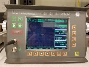
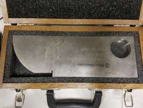
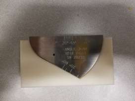 Figure 2 Figure 3
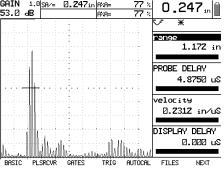
Figures 1 shows the GE Inspection technologies Portable Ultrasonic Flaw DetectorUSN 60 used within the laboratory.
Figure 4
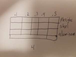
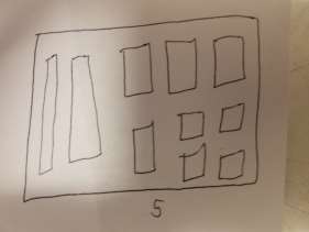
Figure 5
Figures 2,3,4,5,6,7 are figures of all the calibration blocks that were used in the laboratory. Figure 3 shows the miniature angle beam calibration block. Figure 2 shows the IIW calibration block. Figure 4 shows the step calibration block in different material types. Figure 5 shows the ASTM calibration kit.
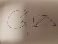
Figure 6
Figure 6 shows the wedges that were used for angle beam calibration and testing. The left block is 45° and the right block is 70°
Figure 7 Figure 8
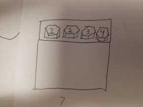
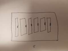
Figure 7 shows the bolts that were tested in experiment 6 and figure 8 shows the steel weld samples that were also tested in experiment 6.
Procedure
In experiment 5 the first section was to setup the device. In the lab manual it says to refer to the device’s manual but in the class the professor showed how to use the device. In this experiment we used a GE Inspection technology Portable Ultrasonic Flaw Detectors USN 60. To start off is to start to program to device to the correct parameters. The measurements were always in inches and the probe was determined under the PLSRCVR button menu. To set the probe if it is a single probe or dual probe we use the DUAL part on the screen to set dual on or off, in these experiments the dual will be off. The same screen will be a PULSER which should automatically be spike. After it was all completed under that tab, the home button was pressed to go back to the main menu screen. The left dial on the side would change the dB. The right dial would change the number the selector was put on. The range is changed so the pulse we are looking for is on the screen and not off the screen. To make sure you are reading the correct pulse you must set the gate over the pulse and the width of the pulse you are trying to read. The pulse should also have about 80 percent of amplitude. After all this setup the device may be begin to start to be calibrated.
To begin to calibrate with the straight beam probe for experiment 5, you must determine which material you will be testing and then pick the correct step block that correlates with that material. Determine if you are using a single or dual probe. In this experiment we used a single probe, so the DUAL should be off. If on the top of the home screen a box does not state the SA, then go to the results tab and make sure it is displayed, then hit the home button and press the autocal button. This will display two important windows of REF1 and REF2, these are programmed to which steps you are going to use on the block, and we picked .4″ and .2″ as the references. The range is set to a length longer than the longer reference point you used to be able to see it on the screen. The frequency on the device should also match the frequency of the probe(s) being used. Put gel on the steps and then place the probe on REF1 which should be the smaller thickness. Press record, make sure your gate is over the first pulse for REF1 and press record again, and then move the probe to the second step, move the gate over the pulse and press record again. If it was done correctly the gate over the last pulse recorded should show the numbered thickness on the step. Also on the home screen the velocity and probe delay should be the same as the material that is being tested. If this is correct then the calibration was a success. A picture of the screen was taken for each calibration specimen.
The next section of experiment 5 is to use the angle beam probe on the IIW block and miniature angle block by using a 45° wedge with a 2.25 MHz probe. To set the angle, go to the home screen and then hit the TRIG button, make sure the angle is set to the same angle the wedge you are using. Press the home button again and then go to the results tab and makes sure the boxes on the top of the screen are set up to display SA, PA, DA, A%A. Press the home button again. Press the autocal tab and set the REF1 to 4″ and REF2 to 9″ to program the device for the IIW block, to program the device for the miniature block then set the REF to 1″ and 4″. Put gel between the transducer and wedge before putting them together. Put gel on the block and then place the probe at the 0° that is marked on the block with the line on the wedge. Do the same steps to record the REF as stated before. The velocity of the shear wave that is used in the angle beam probe should be divided by about 2 for the velocity of the longitudinal wave that is used in the straight beam probe in the same specimen. Pictures are taken with the gate over the 4″ and 9″ pulse for the IIW and the 1″ and 4″ pulse for the miniature block.
The final part of experiment 5 was to find the area amplitude and the distance amplitude by using the cylinders from the ASTM set. These cylinders have the same height but the diameters of the hole within the cylinders are different. On the cylinders used the diameters were stated, which we used the cylinders that said 3/64″, 5/64″, and 8/64″. In order to make the graph area vs. amplitude, the equation = 20 was used with the found gain. To determine the distance the six cylinders that had the same diameter hole within in it was used but the height of each cylinder was different which were 1″, 1.25″, 1.5″, 2.25″, 3.75″, and 6.75″. In order to make the graph distance vs. amplitude, the equation = 20 was used with the found gain..
In experiment 6, the initial part was to find the depths of four bolts that are hidden from sight in a box with only the head of the bolt shown. In addition on the bolts we had to determine if the bolt had a defect and the location of the defect. To start, the device must be calibrated by using the straight beam probe method. Put the gel on the top of the bolt and use the 5 MHz probe, make sure the device is set on dual probe on for this probe. While scanning the top of the bolt the pulses on the screen should show the bottom of the bolt which will determine how long the bolt is, also before the pulse for the bottom, other pulses will determine if a defect was found and how far it is from the top of the bolt. Each bolt had a picture taken of the device’s screen to show the defect. After testing the bolts, the next section was to use the 6 dB drop method as described before to seek and locate the appearance of the defect within the random aluminum specimen given. By calibrating the device using the straight beam method and covering the entire surface of the specimen with gel. The specimen was then examined with a horizontal and vertical motion with the probe to locate the defect. While this was happening another person was watching the screen to make sure a pulse was not missed. The pulse would have two equal pulses when a defect was found, after a defect was found, the end was found on and a pencil mark was placed. Each time we found an edge we placed a pencil mark. After we have decided we have found all the edges we would connect the dots to make the shape. After the shapes were decided upon, the back plate was removed and shown the real shapes of the defects, then comparing the drawn shapes wo the actual shapes.
In experiment 6, the welding method was used to examine six welded steel specimens. To begin with start to calibrate the device for the angle beam probe using the procedures as stated before. Following those procedures, apply gel to the surface of the plate being tested and to search for the defect within the welded part of the plate by determining the depth in the specimen compared to the thickness of the specimen. Marking each end of the defect then measuring the length of the defect, then to compare it to the given sheet that will be shown in the appendix, of the defect area. Also stated on the sheet, each length of the defect should be 1 inch in length.
DATA
Experiment 5
Figure 9 Straight pobe Steel .4
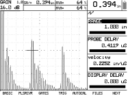
Figure 10 Straight pobe Steel .3
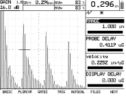
Figure 11 Straight pobe Steel .2
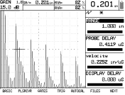
Figure 12 Straight pobe Steel .5
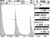
Figure 13 Straight pobe Steel .75
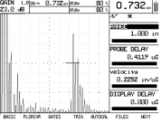
Figure 14 Straight pobe Acrylic .4
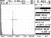
Figure 15 Straight pobe Acrylic .5
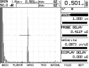
Figure 16 Straight pobe Acrylic .3
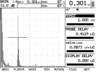
Figure 17 Straight pobe Acrylic .2
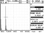
Figure 18 Straight pobe Acrylic .75
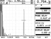
Figure 19 Straight pobe Al .4
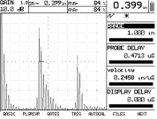
Figure 20 Straight pobe Al .5
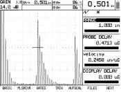
Figure 21 Straight pobe Al .3
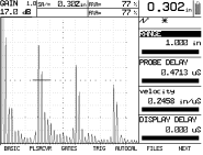
Figure 22 Straight pobe Al .2
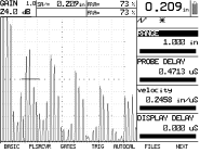
Figure 23 Angle beam , ref 1
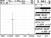
Figure 24 Angle beam, ref 2
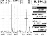
Figure 25 Miniature Angle Beam, ref 2
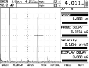
Figure 26 Miniature Angle beam, ref 1
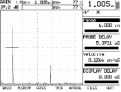
Figure 27 Miniature angle beam reverse, ref 1
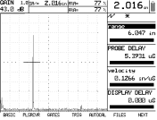
Figure 28 Miniature angle beam reverse, ref 2
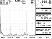
Figure 29 Bolt 1 defect
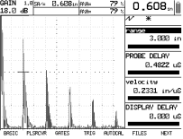
Figure 30 Bolt 1 length
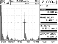
Figure 31 Bolt 2 edge
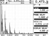
Figure 32 Bolt 2 Length
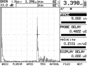
Figure 33 Bolt 3 Length
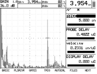
Figure 34 Bolt 3 edge
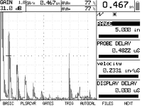
Figure 35 Bolt 4 Length
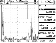
Figure 36 Bolt 4 Defect
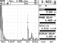
Figure 37 Cylinder 3/64 back wall
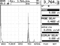
Figure 38 Cylinder 3/64 diameter of flat bottom

Figure 39 Cylinder 5/64
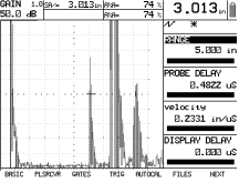
Figure 40 Cylinder 8/64
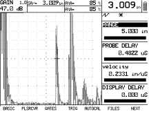
Figure 41 cylinder height 6
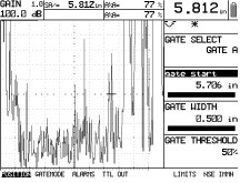
Figure 42 cylinder height 3
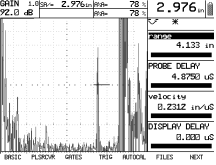
Figure 43 cylinder height 1.5
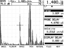
Figure 44 cylinder height .75
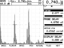
Figure 45 cylinder height .5
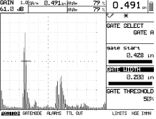
Figure 46 cylinder height .25
Analysis of Data
Part of experiment 5, in straight beam probe calibration, figures 9 through 24 shows pictures of the device screen of a few steps that we used to calibrate the device. For example in steel at .4″ the probe delay was .4119us and velocity was .2252 in/us. In figure 14 the Plexiglas was on stop .4″ with a velocity of .0873 in/us and the probe delay was .4119 us. In figure 19 it sows the .4″ step for aluminum, which shows a velocity of .2458 in/us and probe delay of .4713 us. In figures 13 and 18 show the side of the step block at .75″ for another step.
In angle beam probe calibration, the figures 23 through 28 show pictures of the screen’s device for those calibrations. Figure 23 and 24 shows the references of the IIW steel calibration block which had a velocity of .1599 in/us and probe delay of 26.4325 us. This value was supposed to be half of the straight beam calibration but it was close enough. In figures 25 through 28 shows the miniature calibration block and the probe delay was 5.3931 us and the velocity was .1266 in/us. This was also compared to the straight beam probe velocity in steel and should be about half. It was close enough to be counted. Looking at the probe delays, it seemed to be reasonable time for the distance it had to go.
In area and distance amplitude calibration the figures 37 through 40 displayed the devices screen of each cylinder tested. Figure 37 shows the back wall of the 3/64″ diameter hole which had a 25dB. In figure 38, it shows the 3/64″ diameter of flat bottom hole at 53dB. In figure 39, shows the 5/64 diameter of flat bottom hole with a 50 dB. In figure 40, shows the 8/64″ diameter flat bottom whole with a 47 dB. Each figure had a probe delay of .4822 us and a velocity of .2331 in/us, which was very close to the velocity reference for steel.
Table 1
|
Diameter |
Notation |
Gain (dB) |
|
3/64″ |
V1 |
53 |
|
5/64″ |
V2 |
50 |
|
8/64″ |
V3 |
47 |
Graph 1
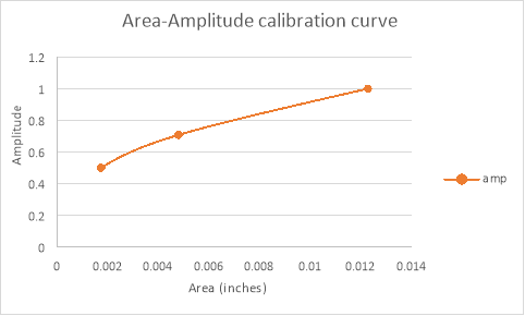
In table 1 it displays the dB for every diameter. In graph 1 the area vs. amplitude calibration curve is shown. Table 1 and equation = 20 was used to calculate the calibration curve. An example of a calculation is shown below:
|V2-V1|=|40 dB – 46dB|= 6 dB
 = 20
= 20 
V2= 2V
In figures 41 through 46, the pictures shown are the different heights of cylinders but the diameter of the hole inside is the exact same. As follows, figure 41 shows 6″ cylinder, figure 42 shows 3″ cylinder, figure 43 shows 1.5″ cylinder, figure 44 shows .75″ cylinder, figure 45 shows .5″ cylinder and figure 46 shows .25″ cylinder. Each figure shows .2312 in/us for velocity and probe delay is 4.8750 us.
|
Notation |
Height |
Sound Path |
Gain (dB) |
|
V1 |
6.75″ |
5.812″ |
100 |
|
V2 |
3.75″ |
2.976″ |
92 |
|
V3 |
2.25″ |
1.480″ |
74 |
|
V4 |
1.5″ |
.740″ |
68 |
|
V5 |
1.25″ |
.491″ |
61 |
|
V6 |
1″ |
.247″ |
53 |
Table 2
Graph 2
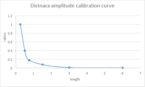
In table 2 it displays the dB and sound paths on the picture taken for each picture of different heights. In graph 2 it displays the distance vs. amplitude calibration curve. The curve was made from the equation = 20 and table 2. If you compare the graph with reference data my graph is not accurate at all. With my data incomplete this is an example of how to calculate the equation:
|V3-V1|=|47.1 dB-97.2 dB|= 50.1 dB
 = 20
= 20 
V3=319.89V
In experiment 6 the bolt defects are shown in figures 29 through 36, which show a picture of the device’s screen for the four bolts that were examined. Figures 29 and 30 for bolt 1 shows the length at 2.03in and defect at .608in, figures 31 and 32 shows bolt 2 with length of 3.398in and defect at .473in, figures 33 and 34 shows bolt 3 with length 3.954in and no defect but we took an edge of the bolt to show, figures 35 and 36 for bolt 4 shows length at 4.426in and defect at 3.922in. Figure 47 shows a picture of the bolts.
Figure 47
- Aluminum Plate defect (6dB drop)-
Figure 48
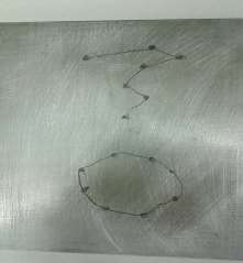
Figure 49
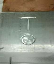
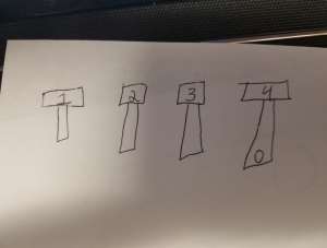
In figures 48 and 49, it displays the aluminum specimen that was tested in experiment 6 using the 6dB technique. Figure 48 shows the sketched markings and figure 49 shows the actual defects.
Figure 50
Defect 1 T= 0.375in length of defect= 1.013in
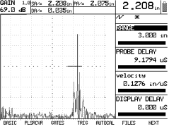
Figure 51
Defect 2 T= 0.395in Length of defect= 1.17in
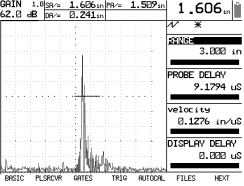
Figure 52
Defect 5 T= 0.397in Length of defect= 1.012in
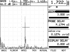
Figure 53
Defect 6 T= 0.390 Length of defect= 0.992
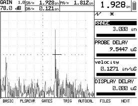
Figure 54
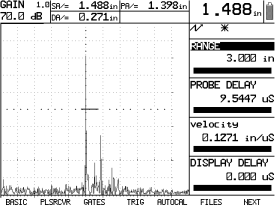
Figure 55
Defect 7 T= 0.390 Length of defect= 1.047
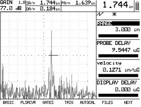
Figure 56
Defect 8 T= 0.389in length of defect= 0.915in
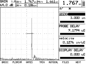
In figures 50 through 56, shows the pictures for the six weld tests examined for experiment 6. Figure 50 shows defect 1 with thickness of .375″ and defect at .035″, figure 51 shows defect 2 with thickness of .395″ and defect at .241″, figure 52 shows defect 5 with thickness of .397in and defect at .201in. Figure 53 and 54 shows defect 6 with thickness of .390″ and defects at .121″ and .271″. Figure 55 shows defect 7 with thickness of .390″ and defect at .184″. Figure 56 shows defect 8 with thickness at .389″ and defect at .186″. This data was compared to the sheet in the appendix.
Discussion of Results
In experiment 5, we learned how to calibrate the three different detector devices using many calibration techniques. One of the methods was straight beam calibration. Following the setup and recording the pictures of the experimental data, we can agree on the calibration was a success. This was agreed by making sure the heights matched the heights of the step block written on the steps. Our heights were very close to the actual height. To make sure this is correct we were also shown a probe delay and velocity. The velocity of steel we got .2252 in/us and the reference velocity was .2300 in/us. The probe delay was .4119 us which was approved by Dr. Genis to be okay. For aluminum the velocity was .2458 in/us and compared to the reference velocity of .2490 in/us, our velocity was very close. The probe delay was .4713 us. For Plexiglas, the velocity was .0873 in/us and compared to the reference velocity .110 in/us was close but still had decent gap. The probe delay was .4119 us.
The next part of experiment 5 was angle beam calibration. Following the setup and recording the pictures of the experimental data, we can agree on the calibration was a success. To see if our data matched was to detect the pulses were in the right place. For IIW calibration block, the first pulse seen was close to the 4″ mark and the second pulse was also very close to 9″ mark. For the miniature calibration block the first pulse was at 1″ and the second pulse was at 4″. We detected all the pulses were at the correct location on the screen. We were also able to get the velocity of .1599 in/us which are approximately half of the reference velocity for steel. The probe delay is 26.4325 us.
In experiment 5, the last part was area amplitude and distance amplitude calibrations. For area amplitude we were able to figure out that we succeeded by the velocity and probe delay. The steel cylinders had a velocity of .2331 in/us, which compared to the steel reference velocity it seems to be very close. The probe delay of .4822 us seemed to match the accepted probe delay. The last part to confirm the data was from graph 1, which shows the area amplitude calibration curve that matched the reference curve that was presented in class. The velocity we obtained was .2312 in/us which was proper. A trend of 7 or 8 in different dB until between two of the cylinders, but at the end it was ok because as long as when the dB was raised the trend line was also being raised. Looking on the graph it seemed that either the graph was wrong or the collected data was wrong.
Cite This Work
To export a reference to this article please select a referencing stye below:
Related Services
View all


DMCA / Removal Request
If you are the original writer of this essay and no longer wish to have your work published on UKEssays.com then please click the following link to email our support team:
Request essay removal