Application of ANN Model
| ✅ Paper Type: Free Essay | ✅ Subject: Engineering |
| ✅ Wordcount: 2038 words | ✅ Published: 30 Aug 2017 |
4.0. Introduction
In this chapter, the results of ANN modelling are discussed through performance parameters, time series plotting and presentation through tables. Before the application of ANN model, statistical analysis of data are done. It is discussed earlier that the selection of appropriate input combination from the available data is the crucial step of the model development process. Five different types of input variable selection (IVS) techniques were utilized and twenty six input combinations were prepared based on the IVS techniques which are discussed in section 4.2. Finally, results of four ANN models are discussed one by one. Firstly, the feed forward neural network model were picked to predict dissolved oxygen of Surma River with all twenty six input combinations and compared with one another. Secondly, the sensitivity analysis was done by changing the value of individual input variables in a certain percentage. Thirdly, six best input combinations were selected based on their performances and rest of the three ANN models were utilized with those selected six input combinations. Finally, three best models from each ANN model were picked to compare with each other. The results of statistical data analysis, results of IVS, and results of ANN models will be discussed in this chapter chronologically.
4.1. Statistical Analysis of Data:
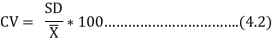
Statistical parameters are very important components to understand the variability of a data set which is prerequisite of any modeling works.This study used some basic statistical parameters i.e. minimum, maximum, mean, standard deviation (SD) and coefficient of variability (CV) as defined below:
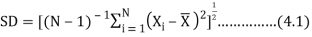
Where, N is the total number of samples,  is the water quality data,
  is the arithmetic mean of that particular data series. The summary of analysis is represented in Table 4.1. Standard Deviation (SD) shows the variation in data set, where smaller value represents the data is close together, while larger value denotes wide spreading of data set. The SD of dependent variable (BOD) showed relatively small value with respect to other parameters. But sometimes it’s difficult to understand variability only by SD value. Thus, coefficient of variability (CV) was used in this study for clear understanding of variability. Value of CV for BOD displayed larger variation (75%) that represents huge quantities of untreated wastewater was dumping from various point and nonpoint sources into this river during sample collection. All independent variables (remaining 14 parameters) also showed an enormous variation in CV value (8% to 144%). Such variability might be happened due to geographical variations in climate and seasonal influences in the study region. pH showed lowest variation and it may happen due to the buffering capacity of the river.
Table 4. 1: Basic Statistics i.e. minimum (min), maximum (max), mean (M), standard deviation (SD) and coefficient of variation (CV) of the measured water quality variables for a period of three years (January, 2010-December, 2012) in Surma River, Sylhet, Bangladesh.
|
Variable |
Min |
Max |
Mean |
Std. |
CV (%) |
|
Phosphate (mg/l) |
0.01 |
3.79 |
0.53 |
0.70 |
132 |
|
Nitrates (mg/l) |
0.18 |
4.0 |
1.53 |
1.05 |
69 |
|
CO2 (mg/l) |
8.0 |
127 |
32.66 |
20.99 |
64 |
|
Alkalinity (mg/l) |
21 |
195 |
59.34 |
30.56 |
51 |
|
TS (mg/l) |
55 |
947 |
292.2 |
165.69 |
57 |
|
TDS (mg/l) |
10 |
522 |
142.3 |
102.15 |
72 |
|
pH |
5.7 |
8.25 |
6.92 |
0.55 |
8 |
|
Hardness (mg/l) |
45 |
262 |
119 |
43 |
36 |
|
SO4-3 (mg/l) |
2.0 |
33.10 |
10.68 |
6.82 |
64 |
|
BOD (mg/l) |
0.6 |
17.3 |
3.79 |
2.86 |
75 |
|
Turbidity (NTU) |
4.18 |
42.62 |
11.84 |
7.37 |
62 |
|
K (mg/l) |
1.47 |
35.22 |
5.45 |
5.75 |
106 |
|
Zinc (mg/l) |
0.1 |
0.52 |
0.19 |
0.09 |
47 |
|
Iron (mg/l) |
0.09 |
6.09 |
0.48 |
0.69 |
144 |
|
DO (mg/l) |
1.9 |
17.30 |
5.40 |
2.45 |
45 |
4.2 Results of input variable selection:
It is mentioned earlier that selection of appropriate input variables is one of the most crucial steps in the development of artificial neural network models. The selection of high number of input variables may contain some irrelevant, redundant, and noisy variables might be included in the data set (Noori et al., 2010). However, there could be some meaningful variables which may provide significant information. Therefore, reduction of input variables or selection of appropriate input variables is needed. There are so many IVS techniques available such as genetic algorithm, Akaike information criteria, partial mutual information, Gamma test (GT), factor analysis, principal component analysis, forward selection, backward selection, single variable regression, variance inflation factor, Pearson’s correlation and so on. In this research, five IVS techniques such as factor analysis, variance inflation factors, and single variable -ANN, single variable regression, and Pearson’s correlation (PC) are utilized to find out appropriate input combinations. The explanation of five selected IVS techniques are explained with the respective input combinations.
4.2.1. Factor Analysis:
Factor analysis is a method used to interpret the variance of a large dataset of inter correlated variables with a smaller set of independent variables. At the initial stage, the feasibility study was carried out for the input variables used in this study was done by KMO index and correlation parameter matrix. The data are suitable for factor analysis if KMO index is greater than 0.5 and correlation coefficient is higher than 0.3. According to Table 4.1, the data are feasible for factor analysis as the KMO index of all data is found as 0.720 (greater than 0.5) and a null hypothesis (p=0.000) indicates a significant correlation between the variables. Moreover, from Table 4.2, many of the correlation coefficient (Pearson’s) between water quality parameters are greater than 0.3 which also confirms the feasibility of water quality parameters for factor analysis. Table 4.3 describes the eigenvalues for the factor analysis with percent variance and cumulative variance. To find out the number of effective factor, factors with Eigen values 1.5 are considered for ANN model. The scree plot of Eigenvalues are illustrated in Figure 4.2. As observed in Figure 4.1, the Eigen values are in descending order and a drop after 2nd factor confirms the existence of at least two main factors.
Table 4.2 Coefficient of KMO and Bartlett test results
|
Kaiser-Meyer-Olkin Measure of Sampling Adequacy |
0.720 |
|
|
Bartlett’s Test of Sphericity |
Approx. Chi-Square |
533.3 |
|
Df. |
78.00 |
|
|
Sig. |
0.000 |
|
Normally, factors having steeper slope are good for analysis whereas factors with low slope have less impact on the analysis. The first two factors cover 64.607% of total variance (Table 4.4). The results of rotated factor loading using Varimax method are tabulated in Table 4.5. The results indicated that the first factor is CO2, Alkalinity and K+, which are the most influential water quality parameter for Surma River. However, hardness, total solid (TS), Fe and total dissolved solid (TDS) are grouped in the second factor.
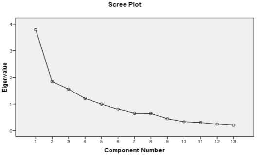
Figure 4.1 Scree plot of eigenvalues of the Surma River
Table 4.4 Individual eigenvalues and the cumulative variance of water quality observations in the Surma River
|
Factors |
Eigen Values |
% Variance |
Cumulative Variance % |
|
1 |
3.800 |
29.227 |
29.227 |
|
2 |
1.839 |
14.147 |
43.374 |
|
3 |
1.553 |
11.947 |
55.321 |
|
4 |
1.207 |
9.286 |
64.607 |
|
5 |
0.997 |
7.668 |
72.275 |
|
6 |
0.802 |
6.172 |
78.447 |
|
7 |
0.645 |
4.965 |
83.412 |
|
8 |
0.639 |
4.914 |
88.326 |
|
9 |
0.442 |
3.400 |
91.727 |
|
10 |
0.331 |
2.548 |
94.275 |
|
11 |
0.304 |
2.341 |
96.615 |
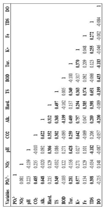
Table 4.5 Rotated factors loading for water quality observations in the Surma River using a Vartimax method
Factor |
NO3– |
pH |
CO2 |
Alk. |
Hard. |
TS |
BOD |
Tur. |
K+ |
Fe |
TDS |
PO4-3 |
||||||||
|
01 |
.070 |
.173 |
.791 |
.876 |
.238 |
.273 |
-.178 |
.443 |
.859 |
-.038 |
.079 |
.179 |
||||||||
|
02 |
.133 |
-.22 |
-.004 |
.143 |
.702 |
.797 |
.007 |
.141 |
.176 |
.621 |
.787 |
.165 |
||||||||
|
03 |
.789 |
-.41 |
-.050 |
-.13 |
.107 |
-.25 |
.152 |
-.526 |
-.010 |
.114 |
-.135 |
.613 |
||||||||
|
04 |
.156 |
.737 |
-.199 |
-.057 |
-.283 |
.117 |
.613 |
.287 |
-.079 |
.416 |
-.162 |
.170 |
Phosphate and nitrate are grouped in factor 3 whereas pH, BOD, Fe are grouped in factor 4. In this research, the variables in the first, second, third and fourth factor are named as the M16, M17, M18 and M19 respectively. All the model names along with their respective variables are tabulated in Table 4.6.
Table 4.6 results of factor analysis with their respective inputs
|
Model |
Input Variables |
|
FA I |
CO2+ Alkalinity + K+ |
|
FA II |
Hardness + TS + Fe + TDS |
|
FA III |
NO3+ PO4 -3 |
|
FA IV |
pH + BOD |
4.2.2. Variance Inflation Factor
The variance inflation factor (VIF) is a method which measure the multi-collinearity in a regression analysis. In this study, variance inflation factors (VIF) were utilized to find appropriate inputs for the proposed model. The performances of VIF are tabulated in Table 4.7. It is found that, the VIF value is not that much satisfactory for all the variables. However, alkalinity, potassium, total solids and phosphate show quite a good result. To prepare some effective input combination for the ANN model, alkalinity was preferred for the model first and all the variables were added one by one. Moreover, only alkalinity is individually not considered in the model as the SV-ANN shows a weak performance for alkalinity (Table 22222). Eleven input combinations were prepared based on the VIF value which is shown in Table 4.8.
Table 4.7 Result of variance inflation factor for individual variables
|
Input Combination |
VIF |
|
Alkalinity (mg/l) |
3.180 |
|
K+ (mg/l) |
2.847 |
|
TS (mg/l) |
2.628 |
|
PO43- (mg/l) |
2.070 |
|
CO2 (mg/l) |
2.036 |
|
TDS (mg/l) |
1.997 |
|
pH |
1.898 |
|
Hardness (mg/l) |
1.820 |
|
Turbidity (NTU) |
1.696 |
|
Fe (mg/l) |
1.290 |
|
BOD (mg/l) |
1.177 |
|
NO3– (mg/l) |
1.175 |
Table 4.8 Results of variance inflation factor (VIF) with their respective inputs
|
Model |
Input Combinations |
|
VIF-I |
Alkalinity + K+ |
|
VIF-II |
Alkalinity + K+ TS |
|
VIF-III |
Alkalinity + K+ TS+ PO4-3 |
|
VIF-IV |
Alkalinity + K+ TS+ PO4-3+ CO2 |
|
VIF-V |
Alkalinity + K+ TS+ PO4-3+ CO2+TDS |
|
VIF-VI |
Alkalinity + K+ TS+ PO4-3+ CO2+TDS+ pH |
|
VIF-VII |
Alkalinity + K+ TS+ PO4-3+ CO2+TDS+ pH+ Hard |
|
VIF-VIII |
Alkalinity + K+ TS+ PO4-3+ CO2+TDS+ pH+ Hard+ Tur. |
|
VIF-IX |
Alkalinity + K+ TS+ PO4-3+ CO2+TDS+ pH+ Hard + Tur. + Fe |
|
VIF-X |
Alkalinity + K+ TS+ PO4-3+ CO2 +TDS+ pH+ Hard + Tur. + Fe + BOD |
|
VIF-XI |
Alkalinity +K+TS+PO4-3+CO2+TDS+pH+Hard+Tur. +Fe + BOD + NO3– |
4.2.3. Pearson’s correlation coefficient
It is not always true that all the variables should contribute to simulate the value of other parameters. Some variables can have a very good relationship with other, some may have weak connection. Pearson correlation is an effective option to understand the relationship with one variable to another. While modelling DO value for the Surma River, it is important to select the variables to have positive relationship with one another. For this reason, a Pearson correlation was prepared which is tabulated in Table 4.3. It is found that there are 4 different types of data combinations which have positive and significant relationship with each other as tabulated in Table 4.9.
Table 4.9 Input combinations using Pearson correlation
|
Model |
Input Combinations |
|
PC I |
Alkalinity + TDS+ PO4-3+CO2+K+ |
|
PC II |
pH + Hardness + Turbidity |
|
PC III |
Alkalinity + Hardness+ TS+CO2+K+ |
|
PC IV |
Hardness+ TS+ K+ Turbidity |
|
PC V |
Hardness+ TS+ Fe +TDS |
|
PC VI |
TS + Turbidity + Fe +TDS + K+ |
4.2.4. SV-ANN
The performance of single variable artificial neural network was also done to find out appropriate input variables for the proposed model. All the individual variables are separately trained, tested and validated. During utilization of SV-ANN, only correlation coefficient (R) is considered to select the appropriate variables. The performances of SV-ANN are tabulated in Table 4.10 for testing, training and validation array. From the analysis, it is found that the individual variables show a weak performance. Only TS and BOD perform better comparing with other variables. The SV-ANN with TS shows a correlation coefficient of 0.596, 0.600 and 0.700 for testing, training, and validation phases respectively. Moreover, the respective correlation coefficient (R) for SV-ANN model with BOD are found as 0.578, 0.574 and 0.652 for testing, training and validation. However, turbidity, carbon di oxide, phosphate and nitrate have quite good relations with DO. As individual variables did not provide significant result, the variables are not considered in the ANN model individually. BOD and TS have quite well
Table 4.10 the correlation coefficient (R) for single variable ANN and single variable MLR
|
Variables |
Phase |
SV-ANN |
SV-MLR |
|
R |
R |
||
|
PO43- (mg/l) |
Testing |
0.439 |
0.115 |
|
Training |
0.549 |
||
|
Validation |
0.440 |
||
|
NO3– (mg/l) |
Testing |
0.211 |
0.148 |
|
Training |
0.311 |
||
|
Validation |
0.112 |
||
|
pH |
Testing |
0.234 |
0.087 |
|
Training |
0.201 |
||
|
Validation |
0.432 |
||
|
CO2 (mg/l) |
Testing |
0.391 |
0.057 |
|
Training |
0.453 |
||
|
Validation |
0.514 |
||
|
Alkalinity (mg/l) |
Testing |
0.222 |
0.200 |
|
Training |
0.211 |
||
|
Validation |
0.099 |
||
|
Hardness (mg/l) |
Testing |
0.139 |
0.089 |
|
Training |
0.649 |
||
|
Validation |
0.155 |
||
|
TS (mg/l) |
Testing |
0.596 |
0.199 |
|
Training |
0.600 |
||
|
Validation |
0.700 |
||
|
BOD (mg/l) |
Testing |
0.578 |
0.100 |
|
Training |
0.574 |
||
|
Validation |
0.652 |
||
|
Turbidity (NTU) |
Testing |
0.431 |
0.183 |
|
Training |
0.583 |
||
|
Validation |
0.398 |
||
|
K+ (mg/l) |
Testing |
0.111 |
0.046 |
|
Training |
0.543 |
||
|
Validation |
0.219 |
||
|
Fe (mg/l) |
Testing |
0.217 |
0.002 |
|
Training |
0.210 |
||
|
Validation |
0.306 |
||
|
TDS (mg/l) |
Testing |
0.222 |
0.084 |
|
Training |
0.345 |
||
|
Validation |
0.245 |
relations with DO so they are grouped in one model (SV-ANN I) and turbidity, carbon di oxide, phosphate and nitrate are grouped in another one (SV-ANN II). The input variables utilizing SV-ANN is tabulated in Table 4.11.
4.3.5. SV-MLR
Like the performances of single variable ANN model, SV-MLR with all the input individual variables show weak performance. Moreover, variables like alkalinity, nitrates, total solid and turbidity show good result comparatively. The performances of SV-MLR are tabulated in Table 4.10. It is found that, alkalinity and TS show quite good results comparing with other variables and hence they are grouped together (SV-MLR I). Another model (SV-MLR II) was prepared using all the variables with correlation coefficient more than 0.200. The input variables using SV-MLR model are tabulated in table 4.12.
Table 4.11 results of single variable artificial neural network with their respective inputs
|
Model |
Input Variables |
|
SV-ANN-I |
TS + BOD |
|
SV-ANN-II |
TS + BOD+ PO4-3+ CO2+Turbidity |
Table 4.12 results of single variable multiple linear regression with their respective inputs
|
Model |
Input Variables |
|
SV- MLR I |
Alkalinity + TS |
|
SV-MLR II |
Alkalinity + TS + Turbidity + NO3– |
|
Model |
IVS Type |
Input Variables |
|
M1 |
PC I |
Alkalinity + TDS+ PO4-3+ CO2 +K+ |
|
M2 |
P Cite This WorkTo export a reference to this article please select a referencing stye below:
Reference Copied to Clipboard.
Reference Copied to Clipboard.
Reference Copied to Clipboard.
Reference Copied to Clipboard.
Reference Copied to Clipboard.
Reference Copied to Clipboard.
Reference Copied to Clipboard.
Related ServicesView allDMCA / Removal RequestIf you are the original writer of this essay and no longer wish to have your work published on UKEssays.com then please click the following link to email our support team: Request essay removalRelated Services Our academic writing and marking services can help you! Freelance Writing Jobs Looking for a flexible role? Study Resources Free resources to assist you with your university studies! |